Population Dynamics and Internal Warfare: A Reconsideration
скачать скачать Авторы:
- Turchin, Peter - подписаться на статьи автора
- Korotayev, Andrey - подписаться на статьи автора
Журнал: Social Evolution & History. Volume 5, Number 2 / September 2006 - подписаться на статьи журнала
ABSTRACT
The hypothesis that population pressure causes increased warfare has been recently criticized on the empirical grounds. Both studies focusing on specific historical societies and analyses of cross-cultural data fail to find positive correlation between population density and incidence of warfare. In this paper we argue that such negative results do not falsify the population-warfare hypothesis. Population and warfare are dynamical variables, and if their interaction causes sustained oscillations, then we do not in general expect to find strong correlation between the two variables measured at the same time (that is, unlagged). We explore mathematically what the dynamical patterns of interaction between population and warfare (focusing on internal warfare) might be in both stateless and state societies. Next, we test the model predictions in several empirical case studies: early modern England, Han and Tang China, and the Roman Empire. Our empirical results support the population-warfare theory: we find that there is a tendency for population numbers and internal warfare intensity to oscillate with the same period but shifted in phase (with warfare peaks following population peaks). Furthermore, the rates of change of the two variables behave precisely as predicted by the theory: population rate of change is negatively affected by warfare intensity, while warfare rate of change is positively affected by population densityKey words: population, warfare, dynamics, nonlinear feedback loops, mathematical models.
INTRODUCTION
The argument that increasing population pressure should lead to more warfare has been made by many social scientists. Malthus (1798), for example, saw war as one of the common consequences of overpopulation along with disease and famine. More recently, the assumption of causal connection between population growth and warfare has served as one of the foundations of the ‘warfare theory’ of state formation (Carneiro 1970; 2000: 182–186; Ferguson 1984; 1990: 31–33; Harner 1970: 68; Harris 1972; 2001: 92; Johnson and Earle 2000: 16–18; Larson 1972; Sanders and Price 1968: 230–232; Webster 1975).
Other anthropologists, on the other hand, express doubts regarding this relationship (Cowgill 1979: 59–60; Redmond 1994; Vayda 1974). For example, Wright and Johnson (1975: 284) pointed out that in South-West Iran by the end of the Uruk Period population declined at the same time as conflict increased. Similarly, Kang (2000: 876) suggested that periods of intensive warfare in protohistoric Korea coincided with underpopulation or depopulation, rather than overpopulation. Finally, a cross-cultural test performed by Keeley (1997: 117–121, 202) did not confirm the existence of any significant positive correlation between the two variables under consideration. The cumulative weight of this critique apparently influenced Johnson and Earle to drop the mention of population pressure as a major cause of warfare in pre-industrial cultures from the second edition of their book (2000: 15–16).
We repeated Keeley's test using the Standard Cross-Cultural Sample database (STDS 2002). The result of this test (Figure 1) would appear to drive the final nail in the coffin of the hypothesis that growing population leads to increased conflict. As we argue in this paper, however, such a conclusion is unwarranted. Our argument is as follows. Both population numbers and warfare intensity are dynamic variables, that is, they change with time. Furthermore, these two variables are dynamically interlinked. Population growth may or may not lead to increased warfare, but warfare certainly has a negative effect on population growth. A more sophisticated version of the population-warfare hypothesis, therefore, would propose that population and warfare are two aspects of a nonlinear dynamical system, in which population growth leads to increased warfare, but increased warfare in turn causes population numbers to decline. One possible outcome of such interaction may be sustained oscillations in which the two dynamic variables cycle with the same period, but phase-shifted with respect to each other (for a nontechnical explanation of the significance of phase shifts, see Turchin 2003b). The theory of nonlinear dynamical systems tells us that we should not necessarily expect a positive linear correlation between the two variables measured at the same time (that is, non-lagged). In fact, depending on the dynamical details of the interaction we may observe a weak positive, a weak negative, or simply no correlation. Thus, in order to empirically test the population-warfare hypothesis we need to use a somewhat more sophisticated approach, which is the subject of this article.
This paper is organized as follows. First, we illustrate our main theoretical point, sketched in the previous paragraph, with an example from non-human population dynamics. Second, we present a general theoretical framework for understanding the interaction between population density and incidence of warfare, and discuss two specific models, one tailored to prestate (and pre-chiefdom) societies, the other appropriate for agrarian states. Third, and most important, we present empirical tests of model-derived predictions addressing historical dynamics in early modern England, Han and Tang China, and the Roman Empire.
Throughout this paper our primary focus is on internal war. In small-scale stateless societies internal warfare occurs between culturally similar groups, and we expect that population dynamics will most directly affect this type of conflict. External war, by contrast, reflects the characteristics not only of the society studied, but also of its alien adversary. In larger-scale societies, such as agrarian states and empires, internal war refers to conflicts ranging from insurrections and revolts affecting a significant proportion of state territory to periods of full-blown state collapse and civil war. The external wars waged by empires appear to have been determined by causes rather different from population pressure. In fact, most historical empires were continuously involved in external warfare aimed at territorial conquest. Furthermore, agrarian empires usually waged external wars with relatively small professional armies. External war mostly affected populations inhabiting borderlands, and had little effect on the demography of central areas. As a result, the negative demographic impact of external war was usually weak, with the exception of infrequent episodes of complete military disasters resulting in the enemy overrunning core areas of the vanquished state. To summarize, the main hypothesis driving this paper is that there is an endogenous dynamical relationship between population dynamics and internal warfare; we treat external warfare as an exogenous variable driven by factors outside our modeling framework. We should also stress that we do not assume that the interaction between population and warfare is the only process that affects the two variables. Real societies are complex systems, and both population numbers and warfare are affected by many other variables, which we treat as exogenous in our modeling framework. The relative strength of the interaction, which we model explicitly, and other – exogenous – factors becomes an empirical issue, to which we will return in the Discussion.
THEORY
An ecological illustration of dynamical interactions characterized by lags
We begin by presenting an ecological example illustrating how the simple-minded approach relying on linear correlation between non-lagged dynamic variables can be very misleading. Our main motivation in using a non-human example is that the basic dynamical concepts are non-controversial, being well established in the ecological literature.
The population interaction between predators and their prey is one of the most common mechanisms underlying population cycles (Turchin 2003a). The simplest model for predator-prey systems was proposed by Alfred Lotka and Vito Volterra in the 1920s (Lotka 1925; Volterra 1926):
 (1)
(1)
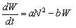
where N and P are population densities of prey and predators, respectively. The first equation says that prey population will increase exponentially in the absence of predators (the term aN), but the presence of predators reduces prey's rate of growth (the term – bNP). The more predators there are, the more prey they kill and the slower prey will increase. Too many predators will result in a negative population growth rate for prey. The second equation says that the more prey there are, the faster will predators increase (the term cNP). The mechanism is simple: predators need to kill and eat prey in order to produce offspring. In the absence of prey (N = 0) predators decline at an exponential rate (the term – dP).
Dynamics predicted by this model are illustrated in Figure 2a. Figure 2b presents the same data as a scatter plot of P against N. The startling result is that there is no correlation between predator and prey density – the regression line is almost perfectly flat. How can that be, since we have explicitly modeled the positive effect of prey density on predators? The answer lies in the fact that predators cannot increase instantaneously in response to high prey numbers – it takes time to give birth to more predators who will eat prey and make even more predators, and so on. In other words, predator population responds to increased prey numbers with a lag. Furthermore, when predators are abundant, they rapidly kill prey off and start starving themselves. But again it takes time for predator population to decline to low numbers. As a result, the positive effect of prey on predator numbers, a mechanism that we have explicitly built in the model, is hidden from us when we use a simple-minded approach of correlating the two variables. But this does not mean that we cannot empirically detect the effect of prey numbers on predators; we just need a better approach.
One way to detect the mechanisms underlying the observed dynamics is to focus not on the structural variables themselves (such as N and P in the Lotka-Volterra model) but on the relationships between the rates of change and the structural variables. For a variety of theoretical and practical reasons, population ecologists usually analyze the rate of change of log-transformed population densities (Turchin 2003a: 25, 184). Define the predator rate of change (on the logarithmic scale) as ∆X(t) = X(t+1) – X(t), where X(t) = log P(t) is the log-transformed density of predators. Plotting ∆X(t) against prey density N(t), we observe a perfect linear and positive relationship (Figure 2c). This should not be surprising, since ∆X(t) is an estimate of dP/(Pdt), and this quantity is linearly related to N by model assumption (see the second Lotka-Volterra equation). Another fruitful approach is to plot one variable against lagged values of the other. For example, if we were to plot P(t) versus N(t−20), we would observe a positive relationship, because the peaks of predator density follow prey peaks with a delay of about 20 years.
We illustrate the theoretical ideas discussed above with a real data from a natural ecosystem (Figure 3). The data document population oscillations of prey, a caterpillar that eats needles of larch trees in the Swiss Alps, and its predators, parasitic wasps. The caterpillar population goes through very regular population oscillations with the period of 8−9 years. Predators (here measured by the mortality rate that they inflict on the caterpillars) also go through oscillations of the same period, but shifted in phase by two years with respect to the prey (Figure 3a). Almost 95% of variation in caterpillar numbers is explained by the model based on wasp predation (Turchin 2003a), but when we plot the two variables against each other we see only a weak, and negative correlation (Figure 3b). If we plot predators against the lagged prey numbers, then we clearly see the positive correlation (Figure 3c).
A model of internal warfare in stateless societies
In this section we extend the insights from the ecological example with a simple mathematical model of internal warfare in stateless societies. Note that we do not propose that the ecological mechanism of predator-prey interaction is of any direct relevance to understanding the dynamics of human societies. Rather, the basic insight has to do with nonlinear dynamics, and is equally applicable to planetary orbits, predator-prey cycles, and, as we hope to show later, the interaction between population dynamics and internal warfare. As we stressed earlier, we focus on internal war (in non-state societies, small-scale warfare between culturally similar groups), because we expect that population dynamics will most directly affect this type of conflict.
The model has two state variables: N, population density, and W, warfare intensity (or frequency). To construct the equation for N we first assume that in the absence of war population will grow logistically. Second, death rate due to warfare is assumed to be directly proportional to warfare frequency. In fact, by appropriately scaling W we can redefine it as the annual warfare death rate, leading to the following equation:
 (2)
(2)
The dynamics of W are governed by two processes. First, we assume that population density causes warfare by increasing the encounter rate between individuals belonging to different groups (‘tribes’). If each tribe sends out foraging parties of a certain size, then the total number of foraging parties is proportional to N. A single party will encounter other parties at the rate also proportional to N. The total number of encounters per unit of time, then, will be proportional to N 2 (the product of total foraging parties and encounter rate per party). Let us assume that each encounter may initiate hostility with a certain fixed probability. Thus, the rate of hostility initiation is aN 2, where a is the proportionality constant.
Second, we assume that the intensity of warfare, in the absence of hostility initiation events, declines gradually at the exponential rate b. This assumption reflects the ‘inertial’ nature of warfare: war intensity cannot decline overnight, even if all objective reasons for it have ceased to operate. In fact, the single most frequent reason for going to war in stateless societies is revenge (McCauley 1990: 9; Wheeler-Nammour 1987). Putting the two processes together we have the following equation:
 (3)
(3)
The term bW in (3) is the rate at which combatants are willing to forget and forgive past injury. It is proportional to W, because high warfare intensity causes greater degree of war fatigue, and therefore greater willingness to de-escalate conflict.
An alternative assumption about hostility initiation is that elevated warfare frequency causes each tribe to send out more war parties. The encounter rate leading to initiation of new conflict, then, will be proportional to the product of population density and warfare intensity (not to population density squared, as in the previous formulation). This assumption leads to the following equation describing the rate of change of W:
 (4)
(4)
We note that the two alternative versions of the population-warfare model, eqns (2) and (3), or (2) and (4), respectively, are structured in a way that is very similar to the Lotka-Volterra predation model. The second model, in particular, differs from the Lotka-Volterra model only in that the population equation has an extra density-dependent term (1–N/K). This should not be surprising, since some historians have already drawn explicit comparisons between warfare and predation (McNeill 1982). We stress again, however, that we do not justify our model by crude analogy with predator-prey interactions; instead we derived it using arguments from first principles.
Mathematical analysis of the two models indicates that they have very similar dynamical behaviors. In particular, both models are characterized by a single equilibrium that is stable for all values of parameters. However, the approach to the equilibrium is oscillatory (Figure 4a). When we plot warfare frequency against population density (Figure 4b), we see a slightly negative, but essentially flat regression line, even though the relationship is completely deterministic. The reason is the same as in the ecological example: high W reflects high N with a lag. When W is high, N cannot remain at a high level: extra mortality resulting from war will result in a population decline. Hence, the periods of significant population growth should coincide with the periods of relatively low warfare frequency, while increase in warfare will lead to population decline, and we will not see a clean correlation between N and W. The appropriate approach for analyzing these data is by focusing on the rates of change. In the model, the population rate of change is affected by warfare negatively, while the warfare rate of change is positively related to population density.
A model of population dynamics – internal warfare in agrarian empires
In large agrarian states (‘empires’) the relationship between population dynamics and internal warfare will be strongly affected by the coercive capacity of the state to impose internal peace, and this factor needs to be taken into account. The model that we discuss here is an extension of the mathematical theory of state collapse discussed in Turchin (2003c: Ch. 7) that incorporates the interaction between N and W modeled with eqns (2−3) in the previous section. Note that the model developed here describes the dynamics of agrarian states, in which the overwhelming majority of inhabitants engage in agriculture.
Let N(t)be the number of inhabitants at time t, S(t)be the accumulated state resources (which we can measure in some real terms, e.g., kg of grain), and W(t) the intensity of internal warfare (measured, for example, by extra mortality resulting from this type of conflict). To start deriving the equations we assume that the per capita rate of surplus production, ρ, is a declining function of N (this is Ricardo's law of diminishing returns) (Ricardo 1817). Assuming, for simplicity, a linear relationship, we have
ρ(N) = c1(1 – N/K)
Here c1 is some proportionality constant, and K is the population size at which surplus equals zero. Thus, for N > K, the surplus is negative (the population produces less food than is needed to sustain it). To derive the equation for N we start with the exponential form (Turchin 2003a):
dN/dt = rN
and then modify it by assuming that the per capita rate of population increase is a linear function of the per capita rate of surplus production, r = c2ρ(N). Putting together these two assumptions, we arrive at the logistic model of population growth:
dN/dt = r0N(1 – N/K) (5)
where r0= c1c2 is the ‘intrinsic rate’ of population growth, and parameter K is now seen to be the ‘carrying capacity’ (Gotelli 1995).
State resources, S, change as a result of two opposite processes: revenues and expenditures. If the state collects a fixed proportion of surplus production as taxes, then revenues equal c3ρ(N)N, where ρ(N)N is the total surplus production (per capita rate multiplied by population numbers), and c3 the proportion of surplus collected as taxes. State expenditures are assumed to be proportional to the population size. The reason for this assumption is that as population grows, the state must spend more resources on the army, police, bureaucracy, and public works. Putting together these processes we have
dS/dt = ρ0N(1 – N/K) – βN (6)
where ρ0= c1c3 is the per capita taxation rate at low population density and β the per capita state expenditure rate.
Internal warfare intensity, W, in the absence of state is assumed to be governed by equation identical to (3):
The presence of state should have a restraining effect on the intensity of internal war. We model this process by assuming that W declines at the rate proportional to state resources, S. Adding this assumption to the equation for W we have:
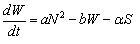 (7)
(7)
The final ingredient is the feedback loop from W to N. High W has a negative effect on demographic rates (birth, mortality, and emigration). In addition to this, internal warfare reduces the productive capacity of the society – fearful of attack, people cultivate only a fraction of productive area, near fortified settlements (a historical example is the movement of settlements to hilltops in Italy after collapse of the Roman Empire [Wickham 1981]). The strong state suppresses internal warfare, and thus allows the whole cultivable area to be put under cultivation. Second, states often invest in increasing the agricultural and general productivity by constructing irrigation and transportation canals, roads, and flood control structures. Intense internal warfare results in deterioration and outright destruction of this productivity-enhancing infrastructure.
We model both effects of W, on the demography and on the productive capacity. First, the demographic effect is modeled by assuming an extra mortality term proportional to W (this is analogous to the derivation leading to Eqn 2). Second, we assume that K, the carrying capacity, is negatively affected by warfare: K(W) = kmax – cW. Putting together all these assumptions we have the following equations:
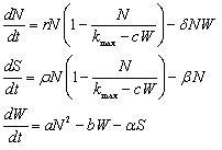 (8)
(8)
All variables are constrained to nonnegative values.
Dynamics of Model (8) are illustrated in Figure 5a. At the beginning of a cycle, both population (N) and state resources (S) grow. Increasing S suppresses internal warfare, with the result that the carrying capacity K(W) increases to the upper limit kmax. At the same time, extra mortality due to warfare declines to zero. As a result, N increases rapidly. However, at a certain population size, Ncrit, well before N approaches kmax, the growth of state resources ceases (the cause of this will be explained in the following paragraph), and S begins to collapse at an increasing rate, rapidly reaching 0. State collapse allows internal warfare to grow, and it rapidly reaches its maximum level. This means that K(W) decreases, and mortality increases, leading to a population density collapse. Population decline eventually allows S to increase again, S suppresses W and another cycle ensues.
The mechanics underlying the relationship between N and S are illustrated in Figure 6. The rate of change of S is determined by the balance of revenues and expenditures. When N is low, population increase results in greater revenues (more workers means more taxes). The growth in state expenditures lags behind the revenues, and state's surplus accumulates. As N increases further, however, the growth in revenues ceases, and actually begins to decline as a consequence of diminishing returns on agricultural labor. However, the expenditures continue to mount. At population density N = Ncrit, the revenues and expenditures become (briefly) balanced. Unfortunately, population continues to grow, and the gap between state's expenditures and revenues rapidly becomes catastrophic. As a result, the state quickly spends the accumulated resources. When S becomes zero, the state is unable to pay the army: the state collapses and internal warfare begins to increase.
The model makes specific predictions about the dynamic interaction between its variables. Because it is difficult to see the trajectory in the three-dimensional space (with axes defined by the state variables N, S, and W), let us define an index of sociopolitical instability as the difference between W and S. Thus, instability grows directly with internal warfare intensity and inversely with state strength. Plotting model-predicted trajectory in the population –instabilityphase space, we see that it traces a periodic attractor (Figure 5b). Again, there is no positive correlation between nonlagged population and instability. Instead, the correlation is slightly negative, and it captures a very small proportion of variance. This general insight, that the interaction between population dynamics and internal warfare (instability) results in coupled oscillations of the two variables, has been tested with a variety of models, including those that explicitly incorporate class structure (see Chapter 7 of Turchin 2003b).
EMPIRICAL CASE-STUDIES
Mathematical theory developed above yields two kinds of general insights. First, it tells us that we should not expect a strong positive correlation between population numbers and warfare intensity (sociopolitical instability). In other words, performing these correlations is the wrong way to test theory. Second, the theory suggests what would be the right way of testing it, because it yields strong quantitative predictions. The theory says that population numbers and internal warfare intensity should oscillate with long periods (ranging from one to three centuries, depending on parameter values), and that these two variables should be phase-shifted with respect to each other. Furthermore, the rate of change of population numbers should be negatively affected by warfare, while the rate of change of warfare should be positively affected by population. To test these predictions we need dynamical data – time-series measures of both population and internal warfare. Such information is hard to come by, but we were able to locate a number of data sets, varying in their accuracy and degree of resolution. Not surprisingly, all empirical case-studies deal with state societies (it is possible that archaeological data on nonstate societies will eventually reach the degree of temporal resolution necessary for testing our theory, but at this point in time we are not aware of any such datasets). We start with the best data coming from late medieval–early modern England, then consider ancient and medieval China, and, finally, the Roman Empire. Our analytical approach is detailed in Endnote 2.
Testing dynamical predictions of the theory with the English data
Our best data set comes from late medieval – early modern England, 1450−1800. Population dynamics of England between 1540 and 1800 have been reconstructed by Wrigley and co-authors (Wrigley et al. 1997; Wrigley and Schofield 1981) using parish records of baptisms, burials, and marriages. This is probably the most accurately known population trajectory in the world prior to 1800 (our analysis stops at 1800 because it was roughly at this date when England made the agrarian-industrial transition, and our theory is specifically focused on agrarian societies). The data for 1450−1530 was taken from Hatcher (1977). To measure sociopolitical instability we compiled all instances of civil war and rebellion during 1450−1800 using the list of Tilly (1993) for the period of 1492−1800, supplemented by Sorokin (1937) for the pre-1492 period and cross-checking with the Encyclopedia of World History (Stearns 2001). A crude, but serviceable index of instability was then constructed by assigning ones to each year in civil war/rebellion, and zeros to all other years. To obtain a more continuously varying measure of instability we smoothed the data with an exponential kernel using bandwidth h = 50 y.
The data indicate that between the late fifteenth century and 1800 England went through several phases in which population growth and sociopolitical instability were in inverse relationship to each other. There were two periods of endemic civil war (the Wars of the Roses of the late fifteenth century, and the revolutionary period of the seventeenth century) during which population stagnated or even declined (Figure 7a, b). There were also two periods of internal stability (roughly, the sixteenth and the eighteenth centuries) during which population grew at a rapid pace. In the phase-plot, the observed trajectory traced out a cycle (Figure 7c). Time-series analysis of these data3 provides strong evidence for reciprocal influences of population and instability on each other (Table 1). In fact, a simple linear time-series model explains a remarkable 85−93 % of variance. Furthermore, the signs of the estimated coefficients (all highly statistically significant, see Table 1) correspond to those predicted by the theory: instability has a negative effect on population, while population has a positive effect on instability. The very tight relationship between the rate of population growth4 and instability is illustrated in Figure 7d.
Han China
We used data on population dynamics reported by Zhao and Xie (1988), and subsequently used by Chu and Lee (Chu and Lee 1994). Zhao and Xie provide estimates of population at irregular intervals; to obtain data sampled at 10-y intervals we interpolated their data with a smoothing exponential kernel (bandwidth = 10 y). Data on sociopolitical instability were taken from Lee (1931), who reported incidence of internal war at 5-y intervals. We smoothed Lee's curve with an exponential kernel (bandwidth = 20 y) and resampled at 10-y intervals, to bring it in line with population series. Both data sets begin with the Han dynasty and continue to the twentieth century. We focused on two periods: 200 BCE – 300 CE, roughly corresponding to the Han dynasty, and 600 – 1000 CE (roughly corresponding to the Tang dynasty). We excluded the 300 – 600 period of political disunity when population estimates are extremely tenuous. The analysis of the post-1000 period is complicated by non-stationarity of population dynamics, and is pursued elsewhere (Korotayev, Malkov, and Khaltourina 2006; Turchin and Nefedov, in prep).
During the Western Han period (206 BCE – 8 CE) population increased from 12 to 60 mln. However, in the first half of the first century China experienced state collapse and rapid growth of internal warfare (including a great peasant insurrection). The result was the loss of at least half of the population (the census of 57 CE found only 21 mln people, Durand 1960). The second cycle, which occurred during the Eastern Han period (25–220 CE), was very similar to the first, but the population collapse was even more catastrophic. Note that two oscillations during the five centuries correspond very well to model-predicted periodicity. What is remarkable is that the index of internal warfare frequency oscillated with the same period, but shifted in phase with respect to population density (Figure 8a).
The trajectory in the N−W phase plot goes through two cycles (Figure 8b). Subjecting these data to the same analysis as the English data, we find that time-series models resolve a smaller proportion of variance (which is not surprising, because these data, and in particular population numbers, were measured with less accuracy than the English ones). Nevertheless, the coefficients of determination fall in the 0.4–0.8 range (Table 1), a very respectable result for what are quite imperfectly measured data. Coefficients associated with reciprocal feedbacks between population and instability are of the correct sign and are all highly statistically significant (Table 1).
The time-series analysis, therefore, strongly suggests that population and instability are dynamically linked. Yet, if we regress log-transformed W(t) on N(t) (the variables plotted in Figure 8b) we find that the relationship is slightly negative. It is statistically significant (F = 4.78, P < 0.05), but explains very little variance (R2 = 0.09). Regressing the rate of change of W on N, however, we obtain a very different result: a simple linear model resolves 72% of variation (Figure 8c), and we now can see that population numbers have a strong positive effect on the warfare rate of change.
Tang China
Data on population and internal war for China between 600 and 1000 were analyzed in exactly the same way as the previous period. The observed dynamics were similar: both variables went through sustained oscillations, with warfare lagging behind population density (Figure 9). Again, coefficients associated with reciprocal feedbacks between population and instability were of the correct sign and are all highly statistically significant (Table 1). The coeficients of determination associated with the fitted time-series models were 0.63−0.64, suggesting that about two-thirds of variance in population numbers and political instability were explained by the feedback effects between the two variables.
The Roman Empire
Population history of the Roman Republic and Empire remains a highly contentious topic (Scheidel 2001). Archaeological data, however, begins to throw light on this obscure aspect of Roman history. Recently Lewit (1991) integrated the results from numerous archaeological sites within the Western Empire, and argued that there were two periods of settlement expansion and two periods of settlement abandonment (Figure 10a). Data on internal warfare in the Roman Empire was published by Sorokin (1937). Plotting the population and warfare data together (Figure 10b) we observe a very interesting pattern. The first century BCE, which was a period of transition between the Republic and Empire, was characterized by intensive internal warfare. During the first half of the Principate (the Early Roman Empire), after internal warfare subsided, population exhibited a long period of sustained growth. The population peak was achieved around 200. During the third century, however, the Empire was convulsed by a series of internal wars, which were accompanied by population decline. Another period of stability and population growth occurred during the first half of the Dominate (the fourth century). After the decline and fall of the Roman Empire in the West, population decreased. Note that Sorokin's index of internal warfare underestimates the extent of actual sociopolitical instability during the fifth century, because he treated barbarian invasions as external warfare.
The estimates of population dynamics are the least satisfactory in this case, and therefore we fitted the time-series model only to instability. Despite the inadequacies of the data, the qualitative dynamics of the variables are clearly consistent with the pattern predicted by the theory: the effect of population index on instability is statistically significant (Table 1).
Testing the results with cross-validation
One potential objection to the analyses we performed is that they require smoothing of data (this is particularly relevant to sociopolitical instability, where the raw data are discrete events). Smoothing introduces autocorrelations between successive observations, while standard statistical tests assume that data points are independent of each other. Furthermore, smoothing may inflate R2, thus overestimating the endogeneity (i. e., signal/noise ratio) of the dynamical process (on the other hand, observation errors bias the endogeneity estimate downward). The most powerful way to address these and other potential statistical problems is cross-validation.
We approached cross-validation by splitting each data set into two equal parts, and then fitting the regression model to the earlier part to predict the latter one, and vice versa. The accuracy of prediction was quantified with the coefficient of correlation between the observed and predicted values (see Supplementary Material for other details).
Cross-validation analysis (see Table 1) showed that including dynamical feedbacks in the models makes them capable of accurately predicting out-of-sample data (that is, data that were not used in estimating model parameters). Most correlations between predictions and observations were over 0.8, and only one was not statistically significant (the only non-significant result was, not surprisingly, for the Roman Empire, the least accurately measured data set). Thus, cross-validation strongly indicates that the relationships detected in our statistical analyses are real.
DISCUSSION
Our main conceptual argument is that population and (internal) warfare are dynamical variables: they change with time and can affect each other. Thus, in order to analyze possible relationships between these variables, we need to use the approaches developed within the nonlinear dynamics theory. In this paper we used both modeling and empirical approaches. The models that we developed here suggest that the dynamic feedbacks between population growth and internal war (or, more generally, sociopolitical instability) should cause coupled oscillations in these variables, with peaks of warfare intensity following peaks of population numbers. Depending on model structure and parameter values, oscillations can either approach a stable equilibrium (as in Figure 4) or continue in a sustained fashion (as in Figure 5). In practice, the difference between oscillatory stability and sustained cycles is not particularly important, because the action of exogenous forces will prevent trajectories from converging to a stable point (or following the limit cycle very precisely), so that in both cases we should observe somewhat noisy sustained cycles. The general results about coupled N −W oscillations is a robust one and does not depend too much on details of model assumptions. Basically, oscillations ensue if both population and warfare are ‘inertial’ variables, and one of them has a positive effect on the other, while the other has a negative effect on the first.
The theoretical result, discussed above, is interesting and suggestive but no more than that in the absence of empirical tests. As we acknowledged in the Itroduction, real societies are extremely complex systems, and both population numbers and warfare are affected by a multitude of other variables (that are exogenous to the models that we discussed in this paper). The empirical issue is whether the coupled interactions between population and warfare generate a strong enough signal to be detected among the ‘noise’ of all other factors acting on societies. Our empirical analyses of historical data suggest that the signal is indeed quite strong, at least in the three or four case studies for which we could find the necessary data. Results of time-series analyses indicate that in all cases but one more than half of variance in population dynamics and warfare intensity was explained by the interaction between these two factors, and in some cases R2 approached the 0.8−0.9 range (see Table 1). In other words, the interaction between population and warfare was the dominant mechanism determining the dynamics of these two variables in the empirical case studies.
This empirical result runs counter to the prevailing mood among anthropologists, who currently tend to de-emphasize the causal connection between population growth and warfare (see Introduction). Concerns raised by earlier workers, however, look much less compelling in the light of theoretical and empirical results in this paper. Thus, observations by both Wright and Johnson and Kang that periods of intensive warfare in southwest Iran and Korea coincided with population declines is precisely what our models predict (see, for example, Figure 5a). Furthermore, Kang's data on the incidence of warfare in the Silla Kingdom suggests that its recurrence was cyclical: peaks in the second-third, fifth, and seventh centuries, interspersed with peaceful fourth, sixth, and eighth centuries (Kang 2000: Figure 3). In other words, warfare recurred approximtely every two centuries, a periodicity which is precisely what our models predict. As Kang noted, at least some of the periods of intense warfare coincided with population declines. It would be interesting to determine whether population grew during the peaceful periods (which is what the theory predicts).
An interesting data set (which is, in a sense, a mirror image of the Korean case because we have good data on population dynamics, but only fragmentary information on warfare intensity) comes from Mesa Verde, Colorado (Figure 11). Frequency distribution of dates when houses were built on Wetherill Mesa suggest that the population there went through four oscillations with the average period of 200 years (ACF signifcant at P < 0.05 level). At least two periods of population decline, the tenth and the fourteenth centuries, were clearly associated with intensive warfare in the archeological record (Varien 1999).
In conclusion, quantitative time-series analysis of several empirical case-studies, ranging spatially across the breadth of Eurasia and temporally over two millennia, suggests that the mathematical theory does an excellent job of capturing dynamic relationships between population dynamics and sociopolitical instability, at least in those cases where we could find appropriate data. Significantly, more precise data resulted in better-resolved relationships (compare the English to the Roman data). It should be stressed, however, that there is one special attribute of all case studies that we analyzed: they all are characterized by a high degree of ‘endogeneity’, and thus it should be easier to detect feedbacks between different variables interacting within these dynamical systems. For example, early modern England was largely insulated from other European states by virtue of its insular position. By contrast, preliminary analysis of the medieval cycle in England reveals a much greater impact of exogenous forces: the effects of the Black Death on population dynamics, and of the cross-channel involvement in French affairs on the rise of instability5. The Roman and Chinese empires were largely ‘closed’ military-political systems by virtue of their size and lack of significant rivals6. In cases involving non-insular medium-sized states and empires, therefore, we would expect to find the relationship between population dynamics and sociopolitical instability to be partially obscured. Despite these caveats, one remarkable finding here was that strong dynamical feedbacks can be detected at all in the historical record. This result has broad implications for the anthropological study of history, suggesting that historical societies can be profitably analyzed as dynamical systems.
NOTES
* This research has been supported by the Russian Foundation for Basic Research (Project № 06-06-80459a) and the Russian Science Support Foundation.
1 The result in Figure 1 is based on the Standard Cross-Cultural Sample (Murdock and White 1969). POPULATION DENSITY CODES: 1 = < 1 person per 5 sq. mile; 2 = 1 person per 1–5 sq. mile; 3 = 1–5 persons per sq. mile; 4 = 1–25 persons per sq. mile; 5 = 26–100 persons per sq. mile; 6 = 101–500 persons per sq. mile; 7 = over 500 persons per sq. mile. WARFARE FREQUENCY CODES: 1 = absent or rare; 2–4 = values intermediate between ‘1’ and ‘5’; 5 = occurs once every 3 to 10 years; 6–8 = values intermediate between ‘5’ and ‘9’; 9 = occurs once every 2 years; 10–12 = values intermediate between ‘9’ and ‘13’; 13 = occurs every year, but usually only during a particular season; 14–16 = values intermediate between ‘13’ and ‘17’; 17 = occurs almost constantly and at any time of the year. DATA SOURCES. For population density: Murdock and Wilson 1972, 1985; Murdock and Provost 1973, 1985; Pryor 1985, 1986, 1989; STDS 2002. Files STDS03.SAV (v64), STDS06.SAV (v156), STDS54.SAV (v1130). For warfare frequency: Ross 1983, 1986; Ember and Ember 1992a, 1992b, 1994, 1995; Lang 1998; STDS 2002. Files STDS30.SAV (v773, v774), STDS78.SAV (v1648–50), STDS81.SAV (v1748–50). STATISTICAL TEST of association between population density and warfare frequency: Rho = 0.04, p = 0.59.
2 We fitted a linear time-series model to the data:
X(t) = a0 + a1X(t–τ) + a2Y(t–τ) + εt (A.1)
(and an analogous model for Y(t)), where X(t) = log N(t) and Y(t) = log W(t) are log-transformed population and internal war index, ai parameters to be estimated, and εt an error term, assumed to be normally distributed (Box and Jenkins 1976). The time delay was τ = 30 y, which approximates the human generation length (but similar results were obtained with an alternative choice of τ = 20 y).
Note that although we used the classical approach of Box and Jenkins, in which the dependent variables are X(t) and Y(t), we have also redone all analyses by using the rates of change of X and Y as the dependent variables. This approach yields very similar results. In fact, statistical tests of reciprocal effects of variables on each other are identical in the two models. This can be seen by substituting the definition of ∆X(t) = X(t) − X(t−τ) into Equation (A.1), as a result of which we obtain
∆X(t) = a0 + (a1–1) X(t–τ) + a2Y(t–τ) + εt (A.2)
3 The analysis of the English data is somewhat complicated by the nonstationarity of population and instability data. We detrended population series by dividing it with estimated carrying capacity, K(t), so that X'(t) ≡ log [N(t)/K(t)], where K(t) is assumed to be proportional to the average wheat yield for the time t. Instability data were detrended by calculating Y'(t) = Y(t) – (a0 + a1t), where a0 and a1 are parameters of linear regression of Y(t) on t.
4 The compound annual growth rate (CGR) was taken from Table A.9.1 of Wrigley (1997) and smoothed using the 25-year running average suggested by Wrigley et al. Note that CGR is also known as the realized per capita rate of population growth; it is the most common measure of population growth used by population ecologists (Turchin 2003a).
5 Export of the ‘surplus elites’ to France during the Hundred Years War reduced social pressures for internal war in England (Bois 1985). It is, thus, not surprising that as soon as the English were finally expelled from France (by 1450), England went into the convulsions of the Wars of the Roses. This analysis will be further pursued in (Turchin and Nefedov, in prep).
6 Even their ‘barbarians’ can be thought of as an integral part of the system. An excellent case for this interpretation of the Chinese – nomad relationship is made by Barfield (Barfield 1989).
REFERENCES
Barfield, T. J.
1989. The Perilous frontier: nomadic empires and China. Oxford, UK: Blackwell.
Bois, G.
1985. Against the neo-Malthusian orthodoxy. In Aston, T. H., and Philpin, C. H. E. (eds.), The Brenner debate: agrarian class structure and economic development in pre-industrial Europe (pp. 107–118). Cambridge: Cambridge University Press.
Box, G. E. P., and Jenkins, G. M.
1976. Time Series Analysis: Forecasting and Control. Oakland, CA: Holden Day.
Carneiro, R. L.
1970. A theory of the origin of the state. Science 169: 733–738.
2000. The muse of history and the science of culture. New York, NY: Kluwer Academic.
Chu, C. Y. C., and Lee, R. D.
1994. Famine, revolt, and dynastic cycle: population dynamics in historic China. Journal of Population Economics 7: 351–378.
Cowgill, G. L.
1979. Teotihuacan, Internal Militaristic Competition, and the Fall of the Classic Maya. In Hammond, N., and Willey, G. R. (eds.), Maya Archaeology and Ethnohistory (pp. 51–62). Austin: University of Texas Press.
Durand, J. D.
1960. The population statistics of China, AD 2–1953. Population Studies 13: 209–256.
Ember, C. R., and Ember, M.
1992a. Codebook for ‘Warfare, Aggression, and Resource Problems: Cross-Cultural Codes’. Behavior Science Research 26: 169–186.
1992b. Resource Unpredictability, Mistrust, and War: A Cross-Cultural Study. Journal of Conflict Resolution 36: 242–262.
1994. War, Socialization, and Interpersonal Violence. Journal of Conflict Resolution 38: 620–646.
1995. War Warfare, Aggression, and Resource Problems: SCCS Codes. World Cultures 9(1): 17–57, stds78.cod, stds78.dat, stds78.rel, stds78.des.
Ferguson, B. R.
1984. Introduction: Studying War. In Ferguson, B. R. (ed.), Warfare, Culture, and Environment. New York: Academic Press.
1990. Explaining War. In Haas, J. (ed.), The Anthropology of War (pp. 26–55). Cambridge: Cambridge University Press.
Gotelli, N. J.
1995. A primer of ecology. Sunderland, MA: Sinauer.
Harner, M.
1970. Population Pressure and the Social Evolution of Agriculturalists. Southwestern Journal of Anthropology 26: 67–86.
Harris, M.
1972. Warfare, Old and New. Natural History 81: 18–20.
2001. Cultural Materialism: The Struggle for a Science of Culture. Walnut Creek, CA: AltaMira Press.
Hatcher, J.
1977. Plague, population and the English economy: 1348–1530. London, UK: Macmillan.
Johnson, A. W., and Earle, T.
2000. The evolution of human societies: from foraging group to agrarian state. 2nd ed. Stanford, CA: Stanford University Press.
Kang, B. W.
2000. A Reconsideration of Population Pressure and Warfare: a Protohistoric Korean Case. Current Anthropology 41: 873–881.
Keely, L. H.
1997. War Before Civilization: The Myth of the Peaceful Savage. New York: Oxford University Press.
Korotayev, A., Malkov, A., and Khaltourina, D.
2006. Introduction to Social Macrodynamics. Secular Cycles and Millennial Trends. Moscow: URSS.
Lang, H.
1998. CONAN: An Electronic Code-Text Database for Cross-Cultural Studies. World Cultures 9(2): 13–56, stds81-2.cod, stds81-2.dat, conan.dbf, conan.dbt.
Larson, L. H.
1972. Functional Considerations of Warfare in the Southeast during the Mississippi Period. American Antiquity 37: 383–392.
Lee, J. S.
1931. The Periodic Recurrence of Intrnecine Wars in China. The China Journal (1931: March–April): 111–163.
Lewit, T.
1991. Agricultural Productivity in the Roman Economy A.D. 200–400. Oxford, UK: Tempus Reparaturm.
Lotka, Al.
1925. Elements of Physical Biology. Baltimore: Williams and Wilkins.
Malthus, T. R.
1798. An Essay on the Principle of Population. London: J. Johnson.
McCauley, C.
1990. Conference Overview. In Haas, J. (ed.), The Anthropology of War. Cambridge, UK: Cambridge University Press.
McNeill, W. H.
1982. The Pursuit of Power. Chicago, IL: University of Chicago Press.
Murdock, G. P., and Wilson, S. F.
1972. Settlement Patterns and Community Organization: Cross-Cultural Codes 3. Ethnology 11: 254–295.
1985. Settlement Patterns and Community Organization: Cross-Cultural Codes 3. World Cultures 1(1): stds03.cod, stds03.dat.
Murdock, G. P., and Provost, C. A.
1973. Measurement of Cultural Complexity. Ethnology 12: 379–392.
1985. Measurement of Cultural Complexity. World Cultures 1(1): stds06.cod, stds06.dat.
Pryor, F. L.
1985. The Invention of the Plow. Comparative Studies in Society and History 27: 740–744.
1986. The Adoption of Agriculture: Some Theoretical and Empirical Evidence. American Anthropologist 88: 894–897.
1989. Type of Agriculture: Variables for the Standard Cross-Cultural Sample. World Cultures 5(3): files STDS54.COD, STDS54.DAT.
Redmond, E. M.
1994. External Warfare and the Internal Politics of Northern South American Tribes and Chiefdoms. In Brumfiel, E. M., and Fox, J. W. (eds.), Functional Competition and Political Development in the New World (pp. 44–54). New York: Cambridge University Press.
Ricardo, D.
181. On the Principles of Political Economy and Taxation. London: John Murray.
Ross, M.
1983. Political Decision Making and Conflict: Additional Cross-Cultural Codes and Scales. Ethnology 22: 169–192.
1986. Political Decision Making and Conflict: Additional Cross-Cultural Codes and Scales. World Cultures 2(2): stds30.cod, stds30.dat.
Sanders, W., and Price, B.
1968. Mesoamerica: The Evolution of a Civilization. New York: Random House.
Scheidel, W. (ed.)
2001. Debating Roman demography. Leiden, Netherlands: Brill.
Sorokin, P. A.
1937. Social and Cultural Dynamics. Vol. III. Fluctuations of Social Relationships, War, and Revolution. New York: American Book Company.
STDS
2002. Standard Cross-Cultural Sample Variables. Edited by Divale, W. T., Khaltourina, D., and Korotayev, A. World Cultures 13(1): files STDS01–88. SAV.
Stearns, P. N.
2001. The Encyclopedia of World History. 6th ed. Boston: Houghton Mifflin.
Tilly, Ch.
1993. European revolutions: 1492–1992. Oxford, UK: Blackwell.
Turchin, P.
2003a. Complex Population Dynamics: A Theoretical/Empirical Synthesis. Princeton, NJ: Princeton University Press.
2003b. Evolution in Population Dynamics. Nature 424: 257–258.
2003c. Historical Dynamics: Why States Rise and Fall. Princeton, NJ: Princeton University Press.
Turchin, P., and Nefedov, S.
in prep. Secular Cycles.
Varien, M. D.
1999. Sedentism and Mobility in a Social Landscape. Tucson: University of Arizona Press.
Vayda, A. P.
1974. Warfare in Ecological Perspective. Annual Review of Ecology and Systematics 5: 183–193.
Volterra, V.
1926. Fluctuations in the Abundance of a Species Considered Mathematically. Nature 118: 558–600.
Webster, D.
1975. Warfare and the Evolution of the State: A Reconsideration. American Antiquity 40: 464–470.
Wheeler-Nammour, V.
1987. The Nature of Warfare. World Cultures 3(1).
Wickham, Ch.
1981. Early Mdieval Italy: Central Power and Local Society, 400–1000. London: Macmillan.
Wright, H.T, and Johnson, G. A.
1975. Population, Exchange, and Early State Formation in Southwestern Iran. American Anthropologist 77: 267–289.
Wrigley, E. A., et al.
1997. English Population History from Family Reconstruction: 1580–1837. Cambridge, UK: Cambridge University Press.
Wrigley, E. A., and Schofield, R. S.
1981. The Population History of England: 1541–1871:a Reconstruction. Cambridge, MA: Harvard University Press.
Zhao, W., and Shujun Zhu Xie
1988. Zhongguo ren kou shi [China Population History] (in Chinese). Peking: People's Publisher.
Supplementary Material
Table 1
Results of time series analyses
|
Source of data |
Dependent variable |
F-statistic for the reciprocal effect1 |
Regression R2 |
Crossvalidation: correlation between data and predictions | |
|
1st half=> 2nd half |
2nd half=> 1st half | ||||
|
England |
population |
137.91*** |
0.93 |
0.90*** |
0.96*** |
|
England |
instability |
76.46*** |
0.85 |
0.92*** |
0.41* |
|
Han China |
population |
15.55*** |
0.42 |
0.86*** |
0.52** |
|
Han China |
instability |
36.47*** |
0.78 |
0.86*** |
0.79*** |
|
Tang China |
population |
50.48*** |
0.64 |
0.76*** |
0.84*** |
|
Tang China |
instability |
13.96*** |
0.63 |
0.80*** |
0.94*** |
|
Roman Empire |
instability |
8.04** |
0.63 |
0.66** |
NS |
1F-statistic of adding the Y(t–τ) term to the X(t) regression in a stepwise fashion, and analogously for the Y(t) regression.
*P < 0.05
** P < 0.01
*** P< 0.001
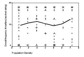
Fig. 1. Relationship between population density and warfare frequency in the Standard Cross-Cultural Sample. Scatterplot with fitted Lowess line. For details of the test, see the Endnote 1.
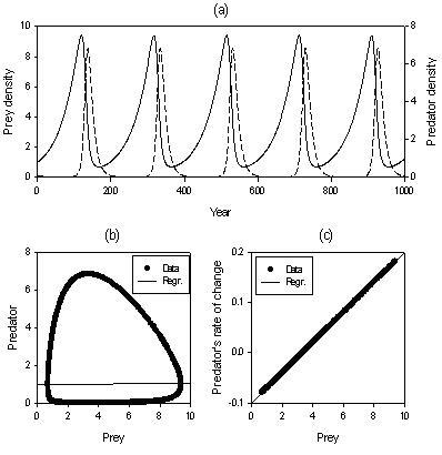
Fig. 2.
(a) Temporal dynamics of prey (solid curve) and predator (broken curve) predicted by the Lotka-Volterra model with parameters a = 0.02, b = 0.02, c = 0.025, and d = 0.1.
(b) The scatterplot of relationship between P and N; the straight line is regression.
(c) The scatterplot of the relationship between the logarithmic rate of change of P (∆p, defined in the text) and N.
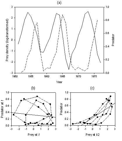
Fig. 3. Population dynamics of the caterpillar (larch budmoth) and its predators (parasitic wasps).
(a) Population oscillations of the caterpillar (solid curve) and predators (broken curve).
(b) A scatter plot of the predator against the prey. The solid line is the regression. Broken lines connect consecutive data points, revealing the presence of cycles.
(c) A scatter plot of the predator against prey lagged by two years.
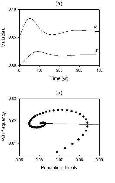
Fig. 4.
(a) A typical trajectory predicted by the model (2–3).
(b) Same trajectory in the phase plot.
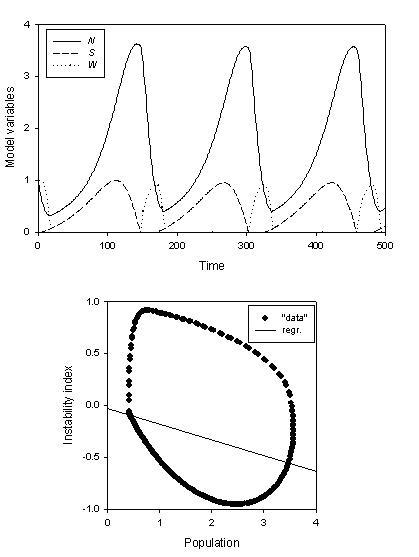
Fig. 5. Dynamics predicted by the Model (8)
(a) Temporal dynamics of population numbers (N), state strength (S), and warfare intensity (W).
(b) The trajectory in the phase space of population and sociopolitical instability (defined as the difference between S and W, see text).
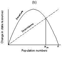
Fig. 6. The mechanics of state collapse
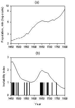
Fig. 7
(a) Population of England, 1450–1800. The broken line indicates less accurately measured data prior to 1540.
(b) Sociopolitical instability in England, 1450-1800. Bars: years in civil war or rebellion. Curve: yearly data smoothed by an exponential kernel with bandwidth of 50 y.
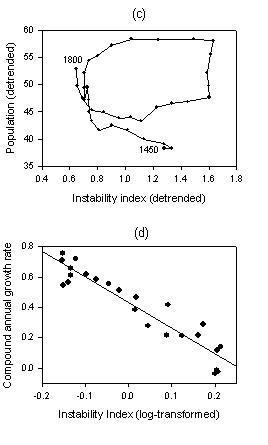
Fig. 7 (cont).
(c) Phase plot (both population and instability are detrended).
(d) Relationship between the per capita rate of population growth and sociopolitical instability in England, 1540–1800.
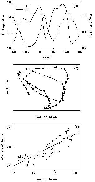
Fig. 8. Analysis of the Han Chinese data.
(a) Population and warfare trajectories.
(b) The trajectory in the population-warfare phase space.
(c) The relationship between the warfare rate of change and population density.
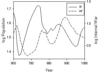
Fig. 9. Dynamics of population and internal war in China, 600–1000.
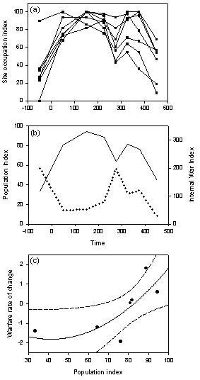
Fig. 10
(a) Relative proportions of excavated settlements occupied during each period in Roman provinces of Britain, Belgica, South and North Gaul, Italy, and South and North Spain.
(b) Population index, constructed by averaging occupation indices in Figure 9a (solid line) and the index of internal warfare (dotted line).
(c) The relationship between the rate of change of internal war and population index. Solid curve: a fitted quadratic regression (broken curves: 95 % confidence intervals).
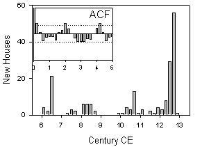
Fig. 11. New houses built on Wetherill Mesa (Mesa Verde area of Colorado, USA) from 600 to 1300 CE. The inset: autocorrelation function indicates a statistically significant periodicity of 2 centuries. Data from (Varien 1999).