The Causal Relation-ship between Remittances and Poverty Reduction in Developing Country: Using a Non-Stationary Dynamic Panel Data
скачать Авторы:
- Gaaliche, M - подписаться на статьи автора
- Zayati, M. - подписаться на статьи автора
Журнал: Journal of Globalization Studies. Volume 6, Number 1 / May 2015 - подписаться на статьи журнала
The aim of this article is to investigate the causal relationship between re-mittances and poverty reduction for 14 emerging and developing countries over the period from 1980 to 2012. We proposed a cointegration analysis, using the method of non-stationary dynamic panel data. Our estimation re-sults reveal that causality nexus of poverty and remittances is bi-directional. We also find that the causal impact of poverty reduction on remittance is stronger than the reverse impact. Indeed, despite of its weak impact on the poverty, remittances should be taken seriously, and this by taking measures by developed countries to facilitate the access of immigrants to their territories. Such an initiative could reduce to some extent the inequalities within developing countries.
Keywords: remittances, poverty, developing countries, cointegration, dynamic panel, causality.
Introduction
International migration is one of the most important factors affecting economic relations between developed and developing countries in the twenty-first century. According to the United Nations, the stock of international migrants estimated is more than 215 million people in 2009, meaning that 3.1 per cent of the world's people were living outside their country of birth (World Bank 2011). The remittances sent back home by migrant workers have a profound impact on the living standards of people in the developing countries of Asia, Africa, Latin America, and the Middle East. In 2012, the flow of international remittances to developing countries stood at $401 billion, a figure which was much larger than total official aid flows to the developing world (World Bank 2013).
The unique characteristics of remittances and their potential economic impact have attracted the attention of policymakers and researchers in recent years, as evidenced by a growing literature aimed at analyzing remittances and their consequences for individual countries. Three main features of remittances provide the impetus for embarking on a study of their macroeconomic impacts: the size of these flows relative to the size of the recipient economies, the likelihood that these flows will continue unabated into the future through continued globalization trends, and the fact that these flows are quite distinct from those of official aid or private capital, which are much better understood in the literature (IMF 2008). These features suggest that the macroeconomic effects of remittances are likely to be substantial and sustained over time and may have unique implications for policymakers in recipient countries.
Remittances reduce poverty through increased incomes, allow for greater investment in physical assets and in education and health, and also enable access to a larger pool of knowledge (Adams 2011). In the past, a number of studies have examined the effect of international migration and remittances on poverty in specific village or country settings (Adams 1991, 1993; Taylor 1992; Gustafsson and Makonnen 1993; Taylor et al. 1999; Stark 1991), but we are not aware of any studies which examine the broader impact of these phenomena on poverty in emerging and developing economies. This paper proposes by using a data set composed of 14 emerging and developing countries, to examine the impact of remittance flows on poverty reduction.
Remittances: Determinants and Limits
A number of factors might determine remittances. Remittances may be motivated by self-interest (Docquier et al. 2007). For example, people might send remittances to enhance their social status or keep a connection with parents in the hope of inheriting their wealth. Remittances could also be viewed as repayments of loans that financed the cost of migration. Lucas and Stark (1985) in examining household data from Botswana found that remittances are positively associated with the wealth of the family left at home. In the literature there is little agreement and scant information concerning the impact of international migration on poverty. Stahl (1982), for example, writes that ‘migration, particularly international migration, can be an expensive venture. Clearly, it is going to be the better-off households which will be more capable of producing international migrants’ (Stahl 1982: 83). Similarly, Lipton (1980), in a study on India that focuses more on internal than international migration, found that ‘migration increases intra-rural inequalities because better-off migrants are “pulled” towards fairly firm prospects of a job (in a city or abroad), whereas the poor are ‘pushed’ by rural poverty and labor-replacing methods’ (Lipton 1980: 227).
Other analysts, however, suggest that the poor can and do benefit from international migration. For example, Stark (1991) finds that in rural Mexico, households are more likely to engage in international migration than are ‘better off’ households. Also, Adams (1991, 1993), in rural Egypt, finds that the number of poor households declines when household income includes international remittances. While the findings of these past studies are instructive, their conclusions are of limited usefulness due to small sample size. Most have addressed individual countries. Clearly, there is a need to extend the scope of these studies to see if their findings hold for a larger and broader collection of developing countries.
Remittances and Poverty: Data Sources and Econometric Model
Our evaluation of the impact of remittances in developing countries is based on an empirical data set that includes data on remittances and poverty for as many developing countries and time periods as possible. The paper uses data from 14 emerging and developing countries1 covering the period from 1980 to 2012. Remittance data were obtained from IMF, Balance of Payments Statistics Yearbook. Indeed, the International Monetary Fund (IMF) keeps annual records of the amount of worker remittances received by each labor-exporting country. However, the IMF only reports data on official worker remittance flows, that is, remittance monies which are transmitted through official banking channels. Since a large (and unknown) proportion of remittance monies is transmitted through private, unofficial channels, the level of remittances recorded by the IMF underestimates the actual flow of remittance monies returning to labor-exporting countries. For the poverty the data were derived from World Bank, more precisely from Global Poverty Monitoring database. In our study, we will use the basic growth-poverty model suggested by Ravallion (1997) and Ravallion and Chen (1997). We propose a four-step analysis with the study of stationarity, cointegration, causality and, finally, decomposition of the variance of the forecast error.
The relationship that they want to estimate can be written as:
log(Pit) = αi + β1 log(μit) + β2 log(git) + β3 log(RMit) + εit (1)
Where:
Pit: is the measure of poverty in country i at time t;
μit: is the per capita real GDP;
git: is the Gini coefficient, it is a measure of the degree of inequality of income distribution in a given society;
RMit: are the remittances to GDP ratio;
εit: is an error term that includes errors in the poverty measure.
To examine the nature of the association between variables, while avoiding any spurious correlation, empirical research in this part follows the four steps: we begin by determining the non-stationarity for all variables. Then, in the second stage, we decide the existence of unit root time series and test the long-term cointegration relationship between the variables. Granted the ratio of long-term, we explore the causal relationship between the variables after determining Granger causality in the third step. In the end, we will study the decomposition of variance.
Econometric Modeling and Results
The results, shown in Table 1, of the unit root tests in the panel are consistent and prove that all variables are integrated of order 1. All series are non-stationary, and it is possible to model through a VAR process. For the four variables, the null hypothesis of no unit root could not be rejected in level. But, in first difference, this hypothesis is rejected for all the variables. Indeed, Fisher's test confirms the most of these results, while Levin and Lin's test come to mixed results. In conclusion, the series in the panel are all integrated of order 1. On the other hand, if we take the two test cases for which the null hypothesis is that of stationarity, we can actually draw the same conclusions as earlier, about the integration of variables from the first difference. Indeed, the null hypothesis of the Hadri's test could not be accepted in level, but it is, in first difference for the variables log(Pit) and log(μit), and in the second difference for the other two variables (log(git) and log(RMit)). This allows us to conclude that, according to Hadri, these two variables are integrated of order 2: I (2).
Table 1
Panel unit root test
| Exogenous variables: Individual effects | |||||||||
| Variable | log(Pit) | Δlog(Pit) | log(μit) | Δlog(μit) | log(git) | Δlog(git) | log(RMit) | Δlog(RMit) | |
| Null: Unit root (assumes common unit root process) | |||||||||
| Levin, Lin & Chu t* | 0.7303 | 3.67379 | –0.3417 | –5.4783 | 4.98460 | 12.5567 | –3.6327 | –11.5975 | |
| (0.8510) | (0.0001) | (0.9314) | (0.0000) | (0.0432) | (0.0021) | (0.0701) | (0.0000) | ||
| Null: Unit root (assumes individual unit root process) | |||||||||
| Im, Pesaran and Shin W-stat | 1.53306 | 1.21116 | –1.00442 | –3.3212 | 0.45077 | 3.43309 | –2.00987 | –6.44089 | |
| (0.8927) | (0.0013) | (0.8780) | (0.0001) | (0.3261) | (0.0003) | (0.3324) | (0.0000) | ||
| ADF – Fisher Chi-square | 10. 5401 | 45.0353 | 5.1117 | 33.1233 | 10.4201 | 40.6004 | 30.9984 | 117.002 | |
| (0.9797) | (0.0006) | (0.6605) | (0.0044) | (0.2506) | (0.0001) | (0.0056) | (0.0000) | ||
| PP – Fisher Chi-square | 1.0872 | 11.3371 | 1.0083 | 25.5544 | 13.0004 | 57.868 | 4.1470 | 77.015 | |
| (0.9987) | 0.0077 | (0.9998) | (0.0006) | (0.3922) | (0.0000) | (0.0052) | (0.0000) | ||
| Null Hypothesis: Stationarity | |||||||||
| Hadri Z-stat | 5.55545 | 0.31129 | 24.7510 | 0.22434 | 8.8334 | 0.99834 | 17.0310 | 2.03325 | |
| (0.0000) | ( 0.4760) | (0.0000) | ( 0.4440) | (0.0000) | (0.0361) | (0.0000) | (0.0551) | ||
| Heteroscedastic Consistent Z-stat | 15.3441 | 1.0105 | 19.3381 | 3.0744 | 9.40693 | 1.96228 | 15.0266 | 9.0229 | |
| (0.0000) | ( 0.4574) | (0.0000) | (0.4411) | (0.0000) | (0.0566) | (0.0000) | (0.0431) | ||
| ** Probabilities for Fisher tests are computed using an asymptotic Chi-square distribution. | |||||||||
| All other tests assume asymptotic normality. | |||||||||
Indeed, since the series are all integrated of order 1, it can be modeled according to a correction error model ‘VECM (p)’. To this end, and to determine the number of lags in our analysis, we estimated various process ‘VAR’ for levels of lags (p) from 1 to 3. For each model, we calculated the Akaike information criteria (AIC), the Schwarz criterion (SIC) as well as the log-likelihood (LV).
Certainly, the results obtained and shown in Table 2 prove that the process to remember is a process with a single lag.
Table 2
Number of lags
| 1 | 2 | 3 | |
| Akaike Info Criterion | –4.114 | –4.1581 | –4.0619 |
| Schwarz Info Criterion | –4.778 | –4.0147 | –2.843 |
| Log Likelihood | 448.58 | 440.61 | 411.542 |
The variables that showed the same order of integration will be used to estimate the cointegrating regression, which justifies the use of cointegration test of Pedroni. The null hypothesis of cointegration test of Pedroni (1999) is the absence of cointegration. The rejection of this hypothesis allows us to conclude the existence of a cointegration relationship between the variables. It should be noted that for small samples, the ADF-Stat built from the ‘between’ model is the most robust. It is this statistic that we use to test the cointegrating relationship between aggregate governance and economic growth. Indeed, under the alternative hypothesis (H1 : ρi < 1, for all i), the value of the Group-ADF tends to –∞, the null hypothesis of no cointegration is rejected for values that tend toward the left tail of the Gaussian distribution. Thus, to 5 per cent, we accept the existence of a cointegration relationship when the Group-ADF statistic is less than –1.645. On the other hand, there are, among the six other statistics, those that tend to +∞ under the alternative hypothesis and we use the positive tail of the normal distribution to reject the null hypothesis. Therefore, these statistics are to be compared to 1.645 at the error threshold of 5 per cent. In conclusion, if the statistics are greater than 1.645 or less than –1.645, then we reject the null hypothesis and accept the fact of existence of cointegration between the variables studied.
The results of the cointegration tests of Pedroni (1999) are shown in Table 3. As can be seen in the overall sample, the seven tests determine the existence of a cointegration relationship between Poverty (Pit) and the explanatory variables. Indeed, the results of the Group-ADF statistic seem to confirm the existence of a cointegrating relationship between remittances and poverty reduction. These results were confirmed also by the test Kao, since the probability of the test is less than 5 per cent and, therefore, we can conclude on the rejection of the hypothesis of no cointegration.
Table 3
Panel Cointegration tests
| Pedroni Residual Cointegration Test | ||||||||||||
| Series: log(Pit), log(μit), log(git), log(RMit) | ||||||||||||
| Alternative hypothesis: common AR coefs. (within-dimension) | ||||||||||||
| Statistic | Prob. | Weighted Statistic | Prob. | |||||||||
| Panel v-Statistic | –140.5657 | 0.8799 | –0.254351 | 0.7744 | ||||||||
| Panel rho-Statistic | 1.811566 | 0.6687 | 1.481106 | 0.6626 | ||||||||
| Panel PP-Statistic | –0.963335 | 0.2336 | 0.213050 | 0.1453 | ||||||||
| Panel ADF-Statistic | –1.023420 | 0.0013 | –2.778401 | 0.0046 | ||||||||
| Alternative hypothesis: individual AR coefs. (between-dimension) | ||||||||||||
| Statistic | Prob. | |||||||||||
| Group rho-Statistic | 9.667691 | 0.9993 | ||||||||||
| Group PP-Statistic | 0.222037 | 0.2307 | ||||||||||
| Group ADF-Statistic | –1.259900 | 0.0002 | ||||||||||
| Kao Residual Cointegration Test | ||||||||||||
| ADF | t-Statistic | Prob. | ||||||||||
| –3.321613 | 0.0000 | |||||||||||
Source: Author's calculation.
At this stage, given that the hypothesis of cointegration is adopted, it is important to determine the number of cointegrating equations using the trace test (Johansen test). In this test, the null hypothesis of no cointegration has been denied in level 2. Table 4 presents the results of this test and shows that there are two cointegrating relationships.
Table 4
Trace test of Johansen
| Hypothesized | Fisher Stat.* | |
| No. of CE(s) | (from trace test) | Prob. |
| None | 443.8 | 0.0000 |
| At most 1 | 166.4 | 0.0000 |
| At most 2 | 17.5 | 0.4384 |
| At most 3 | 97.2 | 0.0000 |
Therefore, for each country in our sample, there are more than one cointegration relationships not necessarily the same for all. Therefore, it is necessary to apply a method of estimating effective. In this context, we will use the FMOLS method (Full Modified Ordinary Least Square) used by Pedroni to clearly specify the long-term relationship that connects poverty reduction in our basic variables and essentially remittances.
Estimation of the cointegrating relationship by fully modified ordinary least square method for different countries in our sample is presented in Table 5 below:
Table 5
Estimation by Fully Modified Least Squares model (FMOLS)
| Pays | log(μit) | log(git) | log(RMit) | C | |||||
| LTU | –1.005*** | 0.972*** | –0.0492 | 14.698 | |||||
| HUN | –0.959** | 1.0018*** | –0.0433 | –13.7731 | |||||
| CZE | –0.9736 | 0.959*** | –0.21803*** | –41.7403** | |||||
| BGR | –1.0122 | 0.977*** | –0.305387* | 12.06455 | |||||
| POL | –0.947 | 1.0025*** | –0.138623 | –13.294 | |||||
| ROU | –0.9754** | 0.989*** | –0.034390 | 0.241209 | |||||
| DZE | –0.941** | 0.975*** | –0.022825 | –2.784636 | |||||
| TUN | 1.094447 | 0.486692* | –0.03298 | –8.7894** | |||||
| EGY | –0.932** | 0.9727*** | –0.08877** | –14.53*** | |||||
| SYR | –0.9439*** | 0.9932*** | –0.064265 | 0.264 | |||||
| SAU | –1.0013*** | 0.965*** | –0.25648*** | –0.737227 | |||||
| MAR | –1.0045*** | 1.00391*** | –0.092470 | –10.72636* | |||||
| IRN | –0.9922*** | 0.927821*** | –0.045009 | 3.56510*** | |||||
| LYB | –0.946751*** | 1.015*** | –0.250286 | –2.354582 | |||||
| PANEL | –1.026108*** | 0.92661*** | –0.09345*** | 1.2139*** | |||||
Note: (***), (**) and (*) show that the corresponding null hypothesis can be rejected respectively at 1 per cent, 5 per cent or 10 per cent.
Source: Authors' calculation.
The above results show that global governance has a negative effect on poverty reduction in all countries and it is more significant pros the following countries: the Czech Republic, Bulgaria, Egypt, and Saudi Arabia. Other countries in the sample have negative but insignificant coefficients. The coefficient in panel of global governance (IGG) is –0.09345 with a Student's statistic equal to 6.22 which implies that the impact of remittances is significantly negative. The coefficients of per capita GDP (income) and the Gini coefficient are consistent with other recent analyses of poverty reduction (Ravallion 1997) and have expected signs.
At this stage, it is essential to estimate the error correction model that will highlight the common cointegrating relationship (common trend) and deduce the interactions between variables. Table 8 summarizes the results for the estimation of equation (2) for poverty reduction.
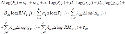 (2)
(2)
Table 8
Estimation of the model with correction of the error for Equation 2
| Dependent Variable: log(Pit) | ||||
| Method: Panel Least Squares | ||||
| Coefficient | Std. Error | t-Statistic | Prob. | |
| C | 3.941662 | 0.770998 | 2.070902 | 0.0198 |
| Δlog(μit) | –0.443684 | 0.037529 | –7.452545 | 0.0000 |
| Δlog(git) | 0.718276 | 0.216257 | 1.795439 | 0.0443 |
| Δlog(RMit) | –0.002062 | 0.019936 | –0.103446 | 0.9007 |
| log(Pit–1) | –0.300183 | 0.054715 | –5.665355 | 0.0000 |
| log(μit–1) | 0.355245 | 0.031695 | 3.856846 | 0.0002 |
| log(git–1) | –0.433607 | 0.097006 | –2.614357 | 0.0077 |
| log(RMit–1) | 0.001515 | 0.014859 | –1.707668 | 0.0981 |
Source: Author's calculation.
According to the spreadsheet, the error term (TCE = α1i) is negative and significant which validates our use of the error correction model. Indeed, the significance of the error correction term validates the existence of a long-term relationship in the process of cointegration, and the movements between different variables are considered permanent. The long-term imbalances between the poverty reduction, the per capita reel GDP, the Gini coefficient and remittances are offset so that the series have similar trends. The value of R2 = = 72.03 per cent shows a good explanatory power of the model. The ‘TCE’ is the speed at which an imbalance between actual and desired levels of poverty is absorbed in the year following any shock. In other words, it corresponds to the automatic stabilizers in the economy. It adjusts 30.01 per cent of the imbalance between the desired and actual level. This percentage is good to stabilize fluctuations in poverty. In case of shocks on remittances and macroeconomic variables, the stabilization process continues and tends to the long term. This explains the volatility of the main aggregates. These aggregates significantly influence the reduction of poverty, both in the short and long term. Moreover, the long-run elasticity's show statistical significances amounting to 1 per cent, 5 per cent and 10 per cent respectively for per capita GDP, Gini coefficient and remittances. While in the short term, the remittances are not significant.
Moreover, the estimated coefficients for per capita GDP and remittances are significantly negative, implying that growth in these factors probably involve a reduction in the poverty especially in the long term in the case of remittances.
In fact, the poverty elasticity's with respect to the per capita GDP (income) and Gini coefficient variables are consistent with other recent analyses of poverty reduction (Adams 2003; Ravallion 1997). The results for the basic specification show that countries with higher income inequality have higher poverty. Indeed, the estimates suggest that, on average, the 1 per cent increase in the income inequality will lead to the 0.443 per cent decline in the poverty headcount in the short term. By cons, any increase of 1 per cent of the Gini coefficient causes an increase in the poor population of 0.718 per cent. For the remittances variable, it has been found that it has a small impact on poverty reduction. In other words, any increases in remittances from immigrants leads to a reduction of 0.0015 per cent of the poverty headcount in the recipient country in the long term.
Thus, we can confirm that remittances have a role in the reduction of poverty in beneficiary's developing countries, but it is still relatively a small-scale compared to the other traditional factors. Indeed, remittances are considered as manna falling from the sky for developing countries, because it represents a free source of income. In this context, with a view to reducing poverty in developing countries, the developed ones should facilitate access of immigrants to their territory. By such a strategy, the recipient country of funds could reduce the burden of poverty on its population without resorting to international aid.
These results have been confirmed by a test of inhomogeneous granger causality on panel data. Indeed, the Fisher test confirmed the rejection of the null hypothesis of homogeneity of non-bidirectional cointegration between remittances and poverty reduction. So there is at least one of the countries in our sample for which there is really a bi-causal relationship between these two factors.
Table 7
Homogeneous Non Causality test in panel
| Pairwise Granger Causality Tests | |||
| Sample: 1980-2010 | |||
| Lags: 1 | |||
| Null Hypothesis: | Obs | F-Statistic | Prob. |
| log(RMit) does not Granger Cause log(Pit) | 462 | 15.0032 | 0.0022 |
| log(Pit) does not Granger Cause log(RMit) | 4.66761 | 0.0246 | |
Source: Author's calculation
Conclusion
In a context where remittances are characterized by a growing trend, the question of the impact of these transfers on the level of poverty did not know yet much investigation, especially in developing countries. For this reason, we have focused our study on a sample of 14 developing countries and on which we have attempted to test the possible relationship of remittances with the poverty headcount. In this case, the analysis confirmed the reducing effect of remittances on level of the poverty rate of the recipient country. Indeed, despite the weak impact of this source of income on reducing inequalities within the recipient country, it represents a way to avoid the dependence of the international aid of the emerging and developing countries.
NOTE
1 Country of Central and Eastern Europe ‘ECO’ and some countries of the MENA region (Middle East and North Africa): Lithuania (LTU), Hungary (HUN), Czech Republic (CZE), Romania, Bulgaria (BGR) Poland (POL), Algeria (DZE), Tunisia (TUN), Egypt (EGY), Saudi Arabia (SAU), Syria (SYR), Morocco (MAR), Iran (IRN) and Lybia (LYB).
REFERENCES
Adams, J. R. 1991. The Effects of International Remittances on Poverty. Inequality and Development in Rural Egypt. Research Report 86. Washington, D.C.: International Food Policy Research Institute.
Adams, J. R. 1993. The Economic and Demographic Determinants of International Migration in Rural Egypt. Journal of Development Studies 30(1): 146–157.
Adams, J. R. 2011. Evaluating the Economic Impact of International Remittances on Developing Countries Using Household Surveys: A Literature Review. Journal of Development Studies 47(6): 809–828.
Docquier, F., Lohest, O., and Marfouk, A. 2007. Brain Drain in Developing Countries. World Bank Economic Review 21(2): 193–218.
Gustafsson, B., and Makonnen, N. 1993. Poverty and Remittances in Lesotho. Journal of African Economies 2(1): 49–73.
Hadri, K. 2000. Testing for Unit Roots in Heterogeneous Panel Data. Econometrics Journal 3: 148–161.
Hurlin, C., and Mignon, V. 2007. Une synthèse des tests de cointégration sur données de panel. Economie et Prévision 4–5: 180–181.
International Monetary Fund. N.d. Balance of Payments Statistics Yearbook. Washington, D.C.
International Monetary Fund. 2008. Macroeconomic Consequences of Remittances. Occasional Paper 259. Washington, DC: International Monetary Fund.
Levin, A., Lin, C. F., and Chu, C. S. J. 2002. Unit Root Test in Panel Data: Asymptotic and Finite Sample Properties. Journal of Econometrics 108: 1–24.
Lipton, M. 1980. Migration from Rural Areas of Poor Countries: The Impact on Rural Productivity and Income Distribution. World Development 8: 1–24.
Lucas, R., and Stark, O. 1985. Motivations to Remit: Evidence from Botswana. Journal of Political Economy 93: 901–18.
Pedroni, P. 1999. Critical Values for Cointegration Tests in Heterogeneous Panels with Multiple Regressors. Oxford Bulletin of Economics and Statistics 61(S1): 653–670.
Ravallion, M. 1997. Can High-Inequality Developing Countries Escape Absolute Poverty? Economics Letters 56: 51–57.
Ravallion, M., and Chen, S. 1997. What Can New Survey Data Tell Us Recent Changes in Distribution and Poverty? World Bank Economic Review 11(2): 357–382.
Stahl, C. 1982. Labor Emigration and Economic Development. International Migration Review 16: 869–899.
Stark, O. 1991. The Migration of Labor. Cambridge, MA: Harvard University Press.
Taylor, J. E. 1992. Remittances and Inequality Reconsidered: Direct, Indirect and Intertemporal Effects. Journal of Policy Modeling 14: 187–208.
Taylor, J. E., Zabin, C., and Eckhoff, K. 1999. Migration and Rural Development in El Salvador: A Micro-Economywide Perspective. North American Journal of Economics and Finance 10(1): 91–114.
World Bank 2011. World Development Indicators 2011. Washington, D.C.: World Bank.
World Bank 2013. Migration and Remittances Factbook 2013. Washington, D.C.: World Bank.
Размещено в разделах