The Punctuated Equilibrium Macropattern of World System Urbanization and the Factors that Give Rise to that Macropattern

ABSTRACT

Change in complex systems, system evolution, is itself complex. This paper is about world system evolution as it is reflected in the pattern of urbanization over the last 5000 years. It will be shown that the pattern of urbanization as part of the immensely complex world system exhibits non-linearity in that it is neither smooth nor continuous but rather is punctuated by periods of rapid change interspersed between periods of stasis. This pattern was first described in biological systems by Eldridge and Gould (1972) for speciation, and much of the pattern of urbanization reflects the characteristics of punctuated equilibrium first described by those two authors. Specifically, this paper will investigate the phenomenon of punctuated equilibrium reflected in both the macro-pattern of urbanization over historic time, i.e. the evidence for punctuated equilibrium as reflected by data on urbanization and on the level of state development, and possible mechanisms for such punctuated behavior including the general model of self-organized criticality as developed by Per Bak (1996), the role of hypercycle formation in punctuated equilibrium, the role of aromorphic processes, and the interaction between population, carrying capacity, and level of technology as represented by a very general math model.

INTRODUCTION

Science is a human endeavor that identifies patterns in nature and then attempts to explain and give predictive value to those patterns by using tested, hypothetical reasoning. History is rightly identified as a branch of science by a number of scholars, chief among them Peter Turchin (2003). This inclusion of history within the domain of science is due to its overlap with the social sciences, is also due to its domain subscribed by the domain of biology, a science, as history is the history of a particular species, our species, Homo sapiens, and finally is due to its being the last segment of a temporal record extending through the domain of paleontology to limits set only by what contemporary cosmology has discovered with that temporal record. All of these conditions are clearly under the scrutiny of a scientific lens, a lens that has been given sharp focus due to the quantitative efforts established by the Russian school of macrosocial dynamics led by Andrey Korotayev and Leonid Grinin and by the efforts of Peter Turchin's newly christened Cliodynamics. Even so, history is only recently coming under formal scientific scrutiny and has much to reveal. [Parenthetically, I would like to point out that the efforts of traditional historians, past and present, is in no way devalued by a more quantitative approach, but that a scientific history is not simply revelatory in its own right but also complimentary and supplementary to the contributions of traditional historians and other social scientists.] It should further be noted that underlying the notions of explanation and prediction is not just a fundamental understanding of phenomenon or pattern but also of mechanism, i.e. how events and processes occur. It is to these ends, to explanation, prediction, and the revelation of mechanism, that this paper is focused, and, more specifically, on the reality of (relatively) abrupt change as it manifests itself in the macro-pattern of urbanization over the last 5000 years of world system history.

As the overarching model applied in this paper is that the human world is a world system, a part of which is the process of urbanization, a note should be made here of the fact that many world system scholars do not agree with the extension backward in time of the existence of the world system to the beginning of urbanization, historical urbanization, at approximately 3000 BCE. Chief among these critics is the doyen of world system analysis, Immanuel Wallerstein, but there are others. The position, however, is taken that the world system, albeit a loosely connected world system, does extend to that temporal horizon, and this position follows the lead of the late Andre Gunder Frank (Frank and Gills 2014) and others who suggest that the world system characteristics of flow of capital, core-periphery structure, and cycles of hegemony and revolution are all evident phenomenon prior to 1500 CE. It is within the context of a world system that the research for this paper was done and done explicitly to address the punctuated pattern of urbanization over the last five thousand years.

Abrupt change in nature has been a subject of scientific study for some time. Phase changes in matter are an obvious example (see, e.g., Sole 2011 and Scheffer 2009) but more recently phase changes have also been identified and investigated in the study of mathematical chaos, in ecological literature, and in a variety of other fields. In 1972 a remarkable paper was coauthored by Niles Eldridge and the late Stephen J. Gould on the reality of punctuated change in the process of speciation. In this paper Eldridge and Gould (1972) showed that a literal interpretation of the evidence of the fossil record in light of the accepted theory of allopatric speciation suggested that the event of speciation was rapid, contra Darwin et al., not stately as the conventional wisdom of gradualism would suggest. The event of speciation itself would occur in small, peripherally isolated populations of a larger biological species population. Lastly the actual event of speciation would consequently hardly ever be subject to preservation in the fossil record. Eldridge and Gould also identified a second reality, that of stasis in the fossil record, and they defined stasis as oscillation about some average value, the oscillations being a result of microevolutionary adjustments to relatively stable local environments. The paper went on to explicitly document examples of punctuation and stasis in both Pleistocene snails and Paleozoic brachiopods, specialty areas of research of both authors. Clearly, this paper, Punctuated Equilibrium: An Alternative to Phyletic Gradualism, was a watershed event with respect to evolutionary understanding and forever changed the context within which evolutionary events would be understood. It was not without controversy.

Eldridge and Gould went further than simply identifying a pattern in the fossil record, they established the reality of biological mechanisms being the motive forces for evolutionary patterns in the record, that is that the fossil record would only reveal pattern in which biological mechanisms, both extant and extinct, created. Specifically in the case of punctuated equilibrium, allopatric speciation was proposed as the mechanism that would produce the stasis and punctuation evident in the fossil record. While it would be inappropriate here to delve into a detailed explanation of allopatric speciation, there are two aspects of that theory which should be brought to the attention of the reader, the geographic distribution of local populations within a given species population and within that distribution the potential for isolation and therefore (relatively) rapid evolution of small, peripheral local populations. These populations would not preserve well in the fossil record but would change rapidly and would therefore represent tipping points in the speciation process. To reiterate, small, (relatively) isolated populations in a species population are potentially subject to rapid change from which new species may arise, an event that is biologically explainable but is not well resolved in the fossil record. Consequently, the temporal distribution of fossils should (and does) reveal both stasis and punctuations. It is a position of this paper that this pattern of (relative) stasis and punctuation occurs by default of context over the course of Big History but is specifically evident in the macro-pattern of urbanization over the last five thousand years of world system history.

A further comment on mechanism is needed here. The late Per Bak (1996), in his research on self-organized criticality, SOC, established a general mechanism for the occurrence of punctuated evolution, and in fact in a brief conversation with Stephen Gould asked if Gould had established a theoretical explanation for punctuated equilibrium, upon which Gould acerbically replied, ‘Punctuated Equilibrium is a theory.’ Sadly, Gould did not recognize the depth of Bak's question, that there had to be a mechanism of a mechanism, that punctuated change required context, constraint, and process in order to occur, and that understood from this broader perspective (the mechanism) would yield greater understanding of the phenomenon of punctuated equilibrium in general. What Bak (1996) describes and Flyberg et al. (1993) proposed by way of mechanism of punctuated equilibrium is simply this; given a set of species with a range of selective values, using a specific selection process, the population of species is upgraded in a way that describes all species surviving above a given threshold selection. This process mimics the pattern of punctuated equilibrium in that periods of stasis (above some minimum selective value) are punctuated by periods of avalanches of change. This biological and theoretical aside is mentioned here, as it will be suggested that the periods of punctuation in urban area evolution over time may have an analogous mechanism. The emphasis here is on ‘may’.

There is one more evolutionary perspective that should be addressed here with respect to the parallel processes of biological and social evolution, that of the Russian school of evolutionary thought. Specifically, the concept of aromorphosis (Grinin, Markov, and Korotayev 2009) has relevance here. Aromorphosis is the evolutionary process by which the evolution of grades of organization occurs. Further, this process can occur relatively quickly and represents a qualitative jump in organization of either a biological or social system. Such events are usually followed by diversification in structure, although the diversification may occur sometime in the future, for example, in biological evolution the origin of the mammalian grade of organization occurred in the Triassic, however the adaptive radiation, that is the diversification of mammals, occurred in the Cenozoic, only after the extinction of (most of) the dinosaurs, which in turn swept the adaptive landscape relatively bare but available for occupation.

It is the position here that the concept of aromorphosis as it applies to social systems has significance with respect to the punctuated phases of urbanization investigated in this paper. After all, urbanization at its base depends on agricultural surplus, a surplus that allows the development of increased social structure and in turn relies ultimately on energy sources to be exploited more efficiently to support that social structure and its evolution. So, there is a positive feedback between the ability to produce food, the efficiency with which the food is produced, the release of human potential to invest in improved technology that will effect population growth and the social organization of that increased (and increasing) population, a fraction of which has been freed from, in fact divorced from, direct food production. Such changes in social structure, that is the evolution of social structure, have not occurred continuously, but exhibit punctuation, and both the details of these aromorphic effects and their mechanisms will be addressed later in this paper.

It should be re-emphasized at this point that while identifying and understanding mechanism is an important goal, the initial and primary intent of this paper is to show that the pattern of stasis and punctuation represents the mode of urban area evolution within the world system, and of course it has also been suggested that this pattern is characteristic of phenomenon within the larger context of Big History, as the concept of punctuated equilibrium certainly occurs well before the advent of cities or even of the genus Homo. However and again, the primary focus of this paper is to show that this punctuated pattern is very much a part of the pattern of urbanization over the last five thousand years.

In order to demonstrate the evidence for punctuation and stasis in the evolution of urbanization within a world system context, modified data for maximum urban area will be used, and in graphical presentation it will be shown that there are three periods of rapid change which are positioned between three periods of stasis. It will further be shown that the three periods of rapid change differ from the periods of (relative) stasis not only in rate of change but also exhibit other characteristics which distinguish them. It will also be shown that associated with the initiation of these periods of rapid change is a threshold ratio value characterizing the level of urbanization at the initiation point of rapid change. Beyond these indicators of change, it will be shown that the nature of the cue to begin periods of rapid change is the existence of a tipping point in the early stages of each of the three periods of punctuation, that is the periods of rapid change, although at present it can only be casually inferred that the tipping points involved are indirect rather than direct. An inference will then be drawn that the change in tempo and mode of urbanization involves an interplay between rural, or at least less urban, and (more) urban populations. Finally, the rudiments of a model mechanism for the alternation between relative stasis and punctuation will be presented, the one which it is hoped will be understood to be at the level of a modest proposal only.

It is important to note here that three papers were previously published, Grinin and Korotayev (2006), Korotayev (2006), and Korotayev and Grinin (2006), each also with quantitative data exhibiting punctuated change. If, for example, one views Diagrams 7, 9, and 10 of Korotayev (2006), Diagrams 1, 3, and 6 of Grinin and Korotayev (2006), or Diagrams 1, 3, 4, 6, 7, and 10 of Korotayev and Grinin (2006) as a representative sample, it can be seen that change over time of the dependent variable in each graph, for example, the number of developed states, world urban population, megaurbanization, particularly for cities with a population larger than 10,000, and territory controlled by developed and states, is not monotonic, in other words not smooth and continuous, but is disjunct with periods of (relatively) rapid change punctuating periods of fluctuation about some mean, all indicative of a pattern of punctuated equilibrium. A more detailed discussion of these findings will be undertaken in a forthcoming paper.

MATERIALS AND METHODS

The data used in this study came from three sources, Chandler's Four Thousand Years of Urban Growth: An Historical Census, World Cities by George Modelski, and the U.S. Census Bureau section on historical demography and are the same sources used in previous investigations (Harper 2010 and others). Both global and maximum urban area population data were natural log transformed to allow graphical comparison over orders of magnitude. The specific data used to demonstrate punctuation and stasis were the continuous accumulation (= summation) of differences between consecutive values of maximum urban area over the last five thousand years of world system history. All graphical representation was done using SciDAVis software, and all regressions were done on a TI-84+ calculator. Further, it is a fundamental assumption of this research that all urban areas exhibit a Pareto/Zipf distribution.

In order to show the distinction between periods of punctuated change and those of relative stasis, it will be necessary first to compare the overall trends in both total world system population and maximum urban area size. Once this has been done, punctuation and stasis will be demonstrated, and it will be shown that these periods quantitatively differ in a disjunct manner. In turn, it will be shown that the periods of quantitative disjunction reveal the presence of unique events associated with them, and in fact these change-motivating events that may be termed tipping points, as they meet a condition associated with tipping points, that of distinct changes in diversity (Lamberson and Page 2012).

Finally, whenever research attempts to penetrate the depths of past time, there is always the criticism that the forces at play then were different than those at play now, permanently obscuring clear knowledge of the past. In fact, beginning with James Hutton and Charles Lyell, this criticism is the basis for the countering notion of uniformitarianism. Historical urban scaling studies (Ortman et al. 2013; Ortman et al. 2014) have shown that the scaled relationships determined for contemporary urban areas also hold for past urban areas. This note is mentioned to underpin the fact that the methods used are applicable over the depth of time studied here.

RESULTS

In Fig. 1A to follow the natural log-transformed data for both maximum urban area and the total world system are plotted against time, and it can be seen that there is general agreement in shape between the two plots.

Specifically, an almost linear plot for total population (top curve) and a less linear but similar trend for the maximum urban area magnitude parallel each other over time up until the beginning of the nineteenth century, point 48 on the x-axis, at which point a steep increase in slope is apparent, being due of course to the early stages of the last phase of the Industrial Revolution (Grinin and Korotayev 2015). At a macro-level these plots are effectively tandem. In further support of this tandemness, when the upper plot, lnT over time, is plotted against the lower plot, lnC_max over time, (Fig. 1B) and a linear regression is generated for the plot, the relationship shown is essentially linear with R² = .9179, the implication of this second graph being that there is a high correlation between the two plots in Fig. 1a. Since the slope of the linear regression in Fig. 1b is slightly greater than one, the rate of growth of urbanization, as characterized by the magnitude of population for maximum urban areas, with the assumption that urban areas of varying (slightly) greater than that of the world system population as a whole.

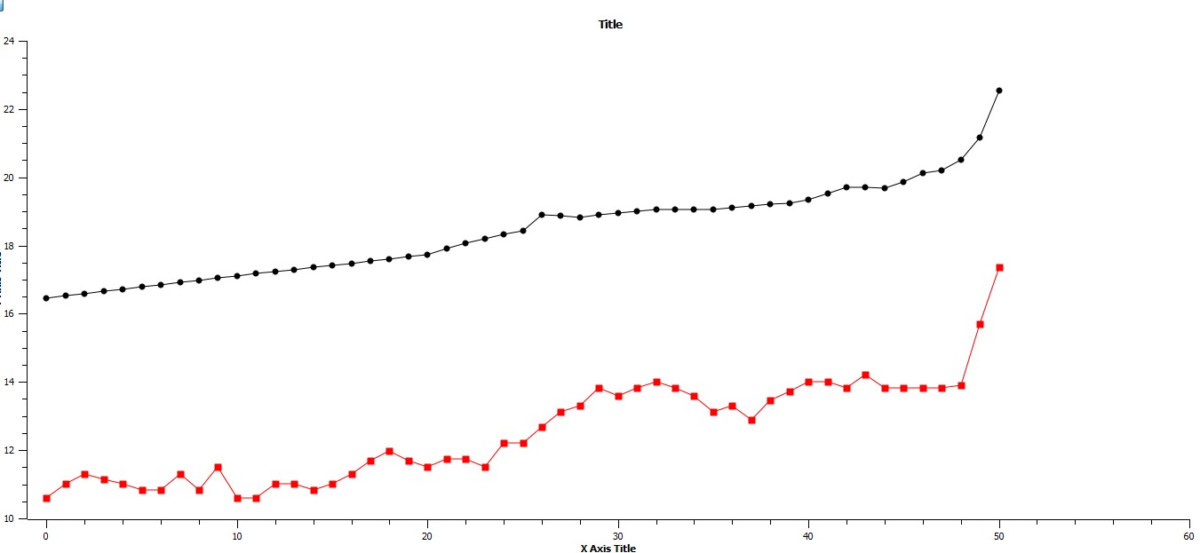
Fig. 1a

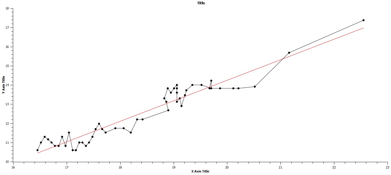
Fig. 1b

1. The x-axis represents time in centuries, and the y-axis represents the natural log-transformed values of both the total world system population, top graph, and the maximum urban area values over the last five thousand years.

2. The x-axis represents lnT, where T = total population of the world system for a given century, and the y-axis represents lnC_max, where C_max = population of the maximum urban area for a given century. The linear regression for this plot is: lnC_max = 1.0700 + 7.1594lnT, R² = .9179.

But there is also evidence for non-linear and non-monotonic behavior of the system as a whole in this second graph, as on closer inspection, the plot of maximum urban area values certainly does exhibit a general tendency of increase but does so with significant and abrupt changes in slope that are both positive and negative. The upper curve does reveal two events of abrupt positive change in slope, one at point 26, that is 400 BCE, for one century which is then followed by a lower slope than the data prior to 400 BCE, and the second at point 48, a population trend that we are currently in and the one aptly described by both Von Forester et al. (1960) and Korotayev et al. (2006). However, the maximum urban area values show more frequent changes, three subsets of which are continuously positive, the first from 1600 BCE to 1200 BCE, the second from 700 BCE to 100 BCE, and the third, which we are, again, currently experiencing, from 1800 CE through to the present (and most probably beyond). Each of these periods of rapid, positive change punctuate periods in which maximum urban area values fluctuate about some mean. It will be shown that these fluctuations appear to have both maximum and minimum values and that each succeeding period of fluctuation does so at a higher average level of maximum urban area population. These periods of fluctuation are analogous to periods of stasis a la punctuated equilibrium in that until conditions occur for rapid increase in maximum urban area values, that is punctuation of the equilibrium, any significant increase in maximum urban area value is relatively shortly followed by a decrease in that value. In other words, the fluctuations in maximum urban area size do so around a mean.

These changes in pattern from ones of fluctuation about some mean and with maximum and minimum limits alternating with continuous and rapid increase are more clearly represented by inspecting the pattern of summed differences in the natural log values of maximum urban area populations. The individual differences in lnC_max from century to century are represented in Fig. 2a, and it can be seen that the values of these differences simply fluctuate about an average value which is above zero but show no indication of alternating periods of stasis and punctuation. Fig. 2b represents the plot of summed differences.

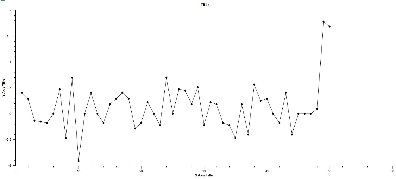
Fig. 2a

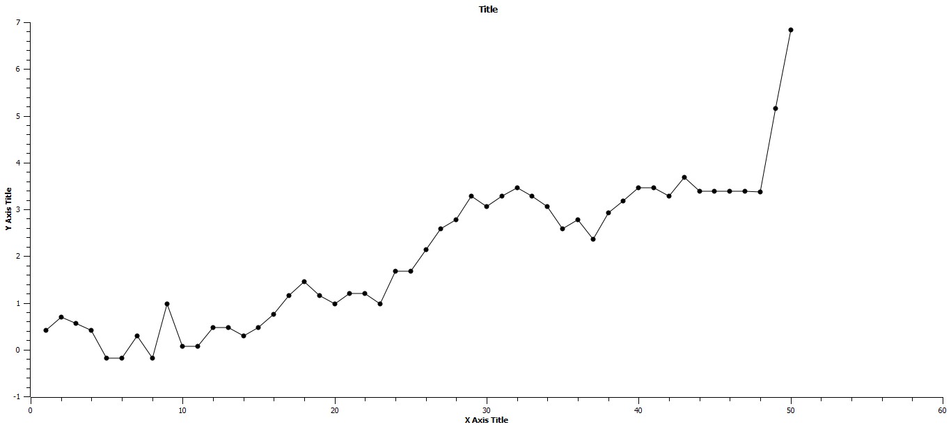
Fig. 2b

1. The x-axis represents time in centuries, and the y-axis represents the differences in maximum urban area values from consecutive centuries. Note that there is no distinction between periods of stasis and periods of punctuation.

2. The x-axis represents time in centuries, and the y-axis represents the summation of the differences in maximum urban area values from consecutive centuries, i.e. ∑∆lnC_max/century. The three periods of rapid change, from 1600 BCE to 1200 BCE, from 700 BCE to 100 BCE, and from 1800 CE through the present, are more prominently represented as are the alternate periods of stasis.

If in turn, these three periods of rapid change and their preceding stasis are represented individually, the change from consecutive phases can be seen even more definitively. In Fig. 3 the period of stasis followed by rapid change are clearly displayed, and linear regressions of each are given. It should be noted that both the slopes and R² values are distinctly different for each. In the prior period of stasis the slope is essentially zero, and the R² value is extremely low, where as in the following period of punctuation the slope is .3020 and R² is .9853, that is that approximately 98 per cent of the variation in the distribution of points is represented by the regression, while the regression for the period of stasis represents almost none of the variation. Considering the next set of stasis and punctuation periods, that is from 1200 BCE to 700 BCE and from 700 BCE to 100 BCE, the same basic pattern is revealed. These data are represented in Fig. 4. Again, as in Fig. 3 both the slopes and R² values are characteristic of each of the consecutive periods of stasis followed by punctuation. Also, the Y-intercept value for this period of stasis is greater than the previous period, that is 2.3378 when compared to .3441, representing a higher plateau, a higher average value for the maximum urban area as a consequence of the previous period of punctuation. The final set of stasis and punctuation periods are represented in Fig. 5 below. As in the previous two sets of stasis followed by punctuation, both the slopes and values for variation are characteristic of their respective time periods, and, further, the Y-intercept value is yet again higher than the previous Y-intercept value, as would be expected due to the period of punctuated growth separating the two periods of stasis.

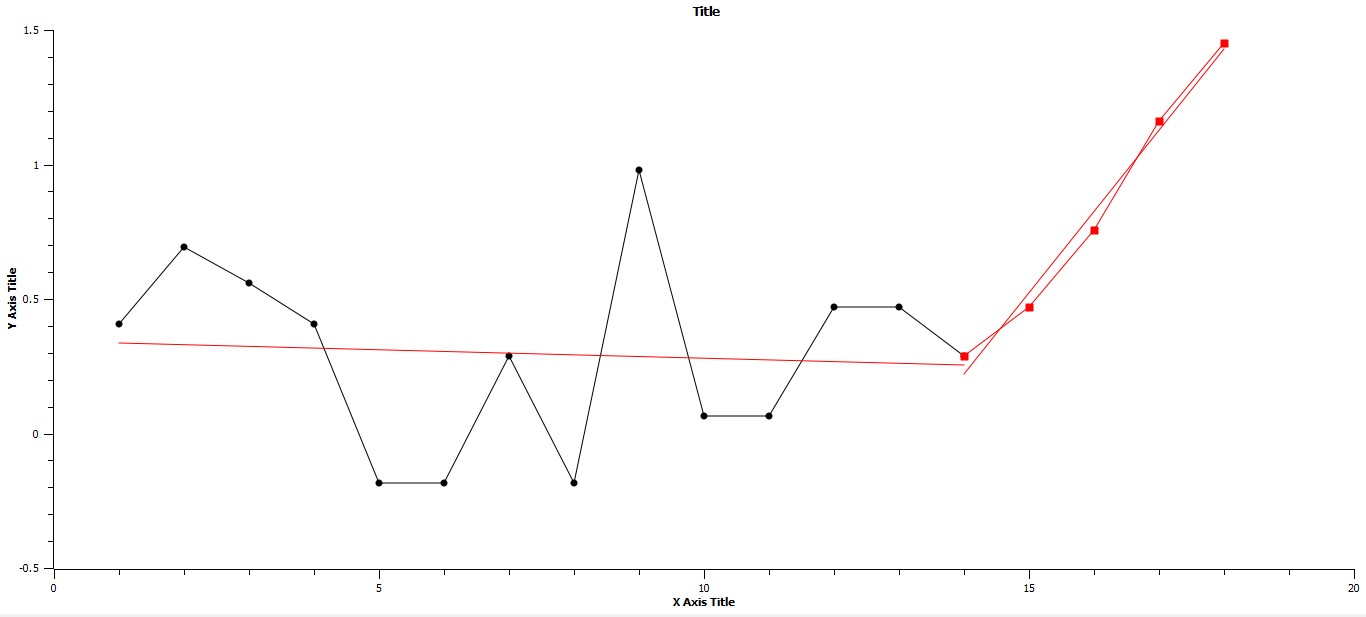
Fig. 3. Axes as in Fig. 2. The linear regressions for the periods, 2900 BCE to 1600 BCE and 1600 BCE to 1200 BCE are respectively: Y = –.0064X + .3441, R² = .0060, and Y = .3040X – 4.0055, R² = .9853

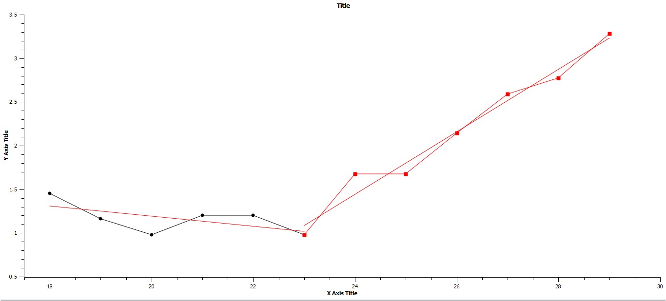
Fig. 4. Axes as in Fig. 2. The linear regressions for the periods 1200 BCE to 700 BCE and from 700 BCE to 100 BCE are respectively: Y = –.0573X + 2.3378, R2 = .3759, and Y = .3579X – 7.1455, R2 = .9732

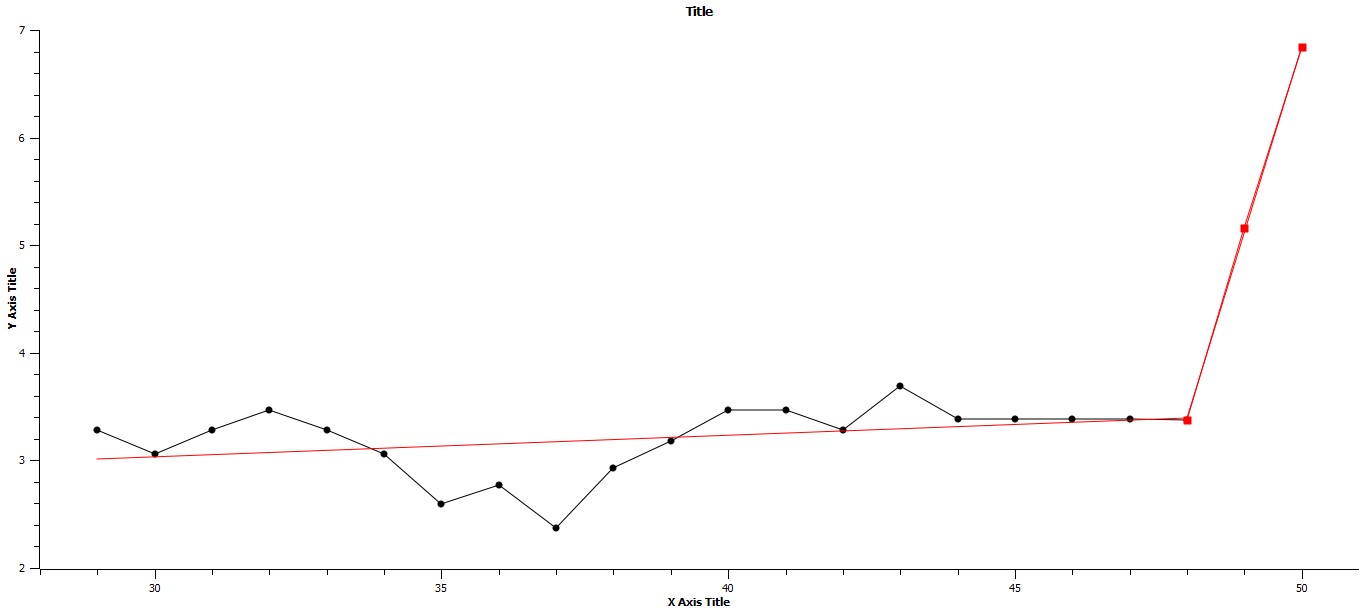
Fig. 5. Axes as in Fig. 2. The linear regressions for periods 100 BCE to 1800 CE and from 1800 CE to 2000 CE are respectively: Y = .0198X + 2.4411, R2 = .1302, and Y = 1.7301X – 79.6479, R2 = .9998

As the previous results imply, there must be some change in the mode of urbanization and the relationship of urbanization to its reverse, this reverse process being labeled ruralization. One line of investigation which will be followed here will be to search for evidence of tipping points, specifically, and these tipping points first occurring from relative stasis to a punctuated mode of urbanization, and then of course whether the tips also exist from a mode of punctuation returning to relative stasis. A tipping point will be understood to be a response to continuous change of a given variable in a discontinuous way, and the evidence for such changes will be a disjunct distribution in diversity on either side of the tip as calculated by: D = ∑1/p², where p represents the frequency of some class of urbanization.

With the previous description of the definition of D in mind, please consider Fig. 6, which represents the distribution of D over the last five thousand years. It is apparent that over the period of time represented that both the magnitude of D and the magnitude of changes in the magnitude of D decrease. Further, there appear to be a number of instances in which D changes precipitously, specifically from 1600 BCE to 1200 BCE almost continuously, from 700 BCE to 600 BCE, and from 1800 CE to 1900 CE. While the change in D from 800 CE to 900 CE appears to represent a significant change visually, it is clear that this peak does not represent a tipping point in which a stasis mode changes to one of punctuation, as it does not occur within the bounds of one of the three periods of punctuation identified previously.

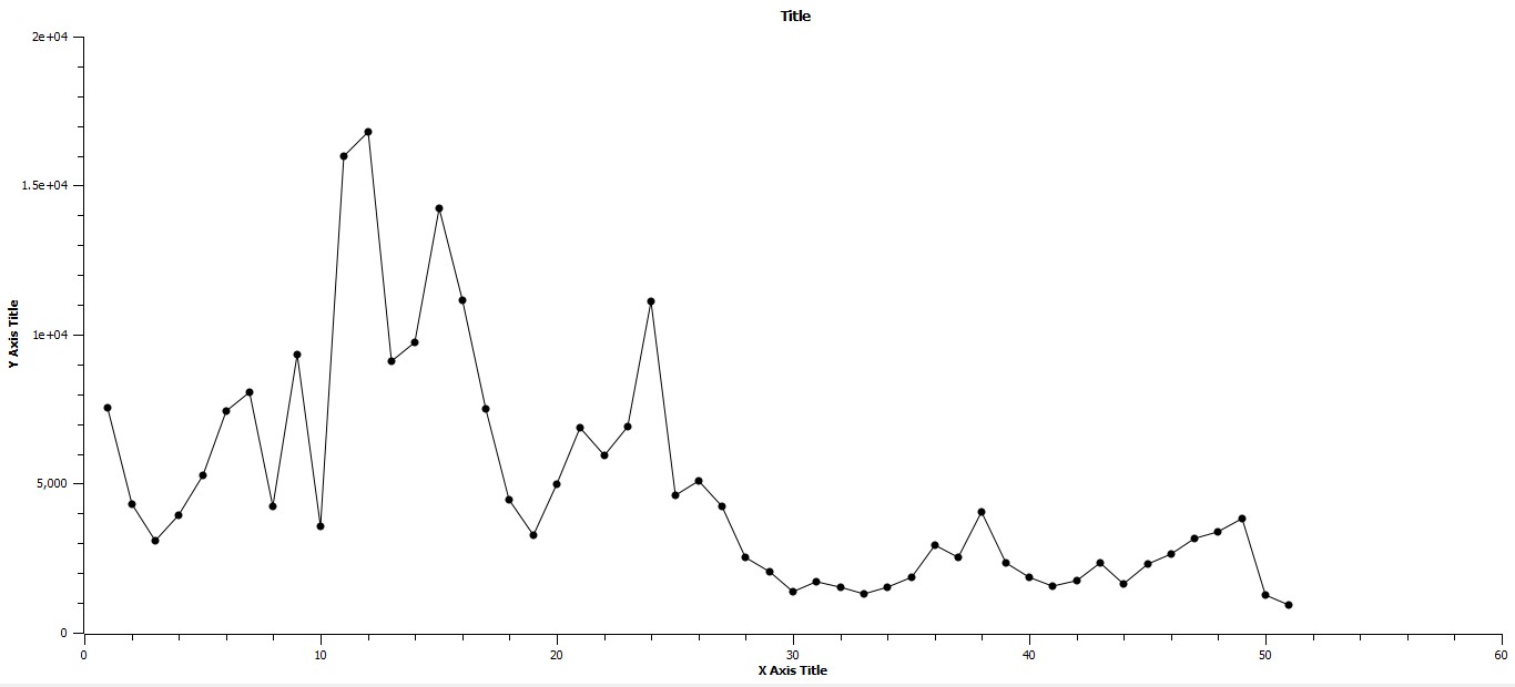
Fig. 6. The X-axis represents time, and the Y-axis represents D. D was computed over a range of values which were fractions of the maximum urban area population for a given century. The graph implies that both the magnitude of changes in D and the absolute values of D decrease with time

Fig. 7 immediately below represents the period of time from 1900 BCE to 1 CE which also includes the period of punctuation from 700 BCE to 100 BCE which marks the shift from the preceding period of stasis, 1200 BCE to 100 BCE, to the following period of stasis, 100 BCE to 1800 BCE. This graphical morphology is consistent with the occurrence of a tipping point. Further, the linear regressions for the three respective time periods have slopes of 1263.1728, –6502.259, and –772.6426. There are two other events meeting the criteria of tipping which are represented in Figs 8 and 9 to follow. Note that Fig. 10 which is a modified form of Fig. 9 is included for completeness, that is to show that the period of 400 hundred years following the impact of the fourteenth century, effectively a reset period where the maximum urban area size is approximately one million, emphasizes the change in the magnitude of D with respect to the succeeding tip period. In both Figs 9 and 10 the pattern of regression is as in Fig. 8 with a positive slope for the period preliminary to the tip period, the very negative slope of the tip period itself, and then a less negative slope for the period succeeding the tip period.

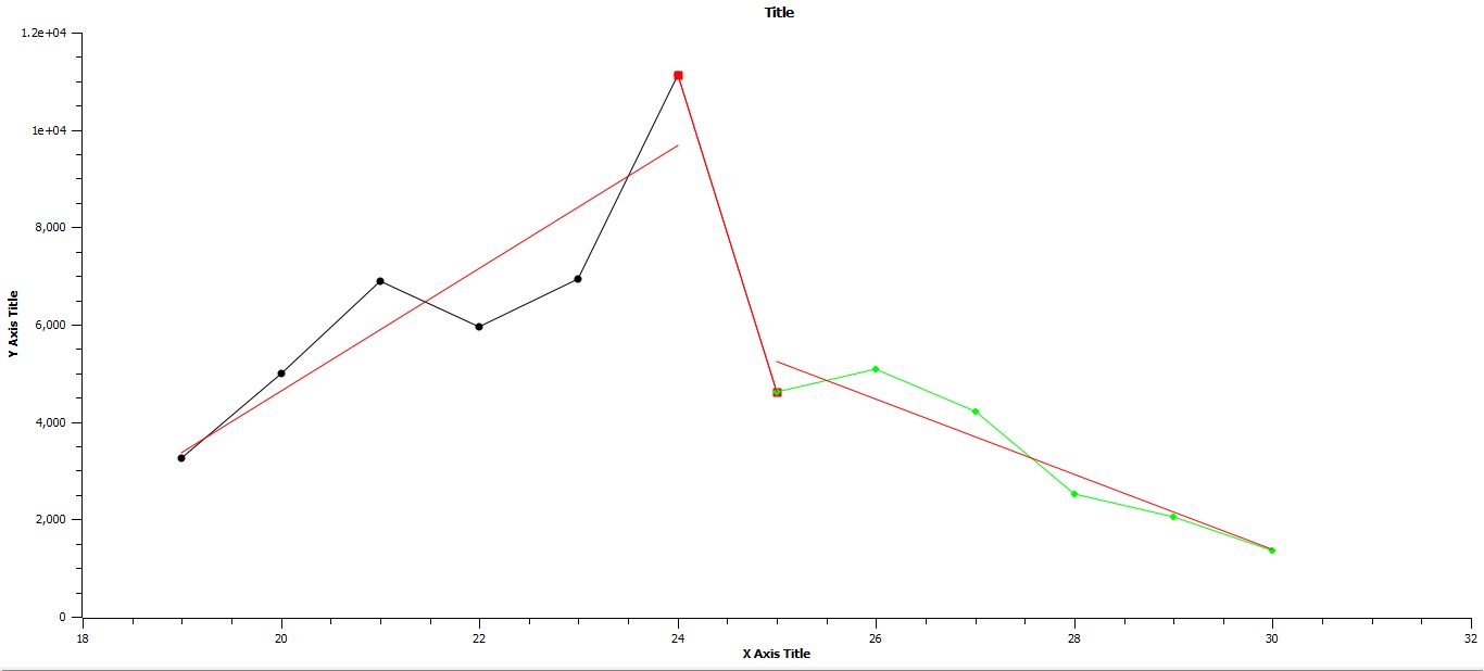
Fig. 7. The X-axis represents time from 1200 BCE to 100 BCE, and the Y-axis represents D. Note that the sequence of regressions from left to right in the graph is respectively: Y = 1263.4141X – 20,633.4141, R² = .8033, Y = –6502.259X + 167,174.305, R² = 1, and –772.6426X + 24,558.0734 R² = .8963, a sequence which would be expected to span a tipping event

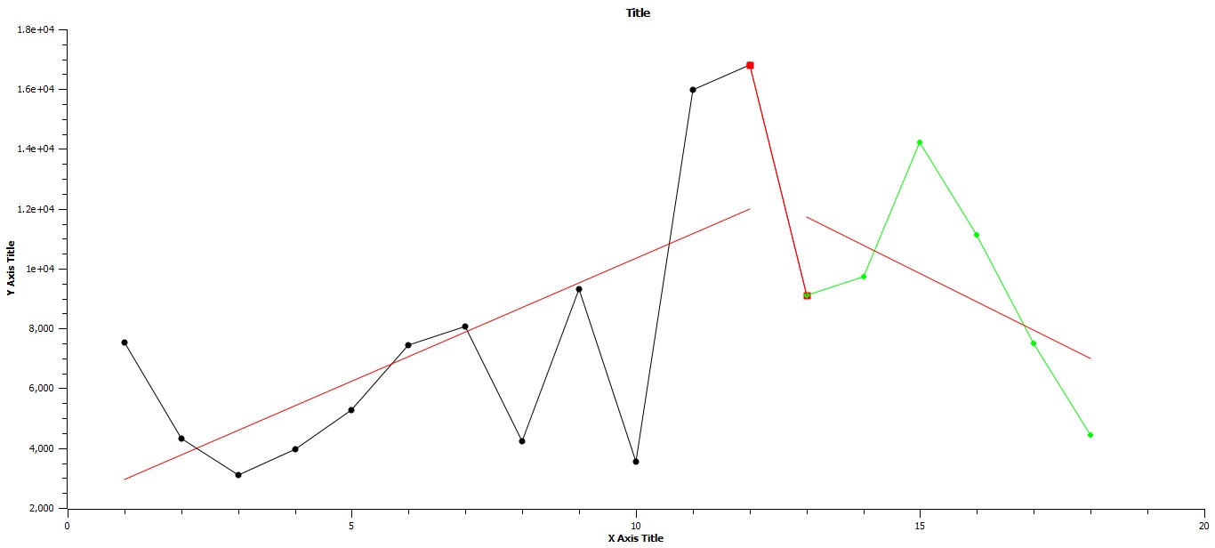
Fig. 8. Axes as in Fig. 7 but over the time span, 3000 BCE to 1200 BCE. Y = 820.5444X + 2134.3555 R² = .4088, –7700.452X + 109,217.86, R² = 1, and –946.5634X + 24033.7208 R² = .2869

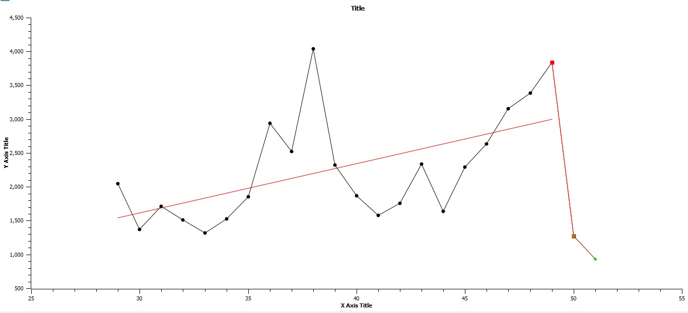
Fig. 9. Axes as in Fig. 8 but over the time span, 100 BCE to 2000 CE. The linear regressions for the periods, 100 CE to 1800 CE, 1800 CE to 1900 CE, and 1900 CE to 2000 CE are respectively: Y = 72.9020X – 574.5061 R² = .3163, Y = –2563.411X – 129,446.947, R² = 1, and Y = –347.759X + 18,644.347, R² = 1

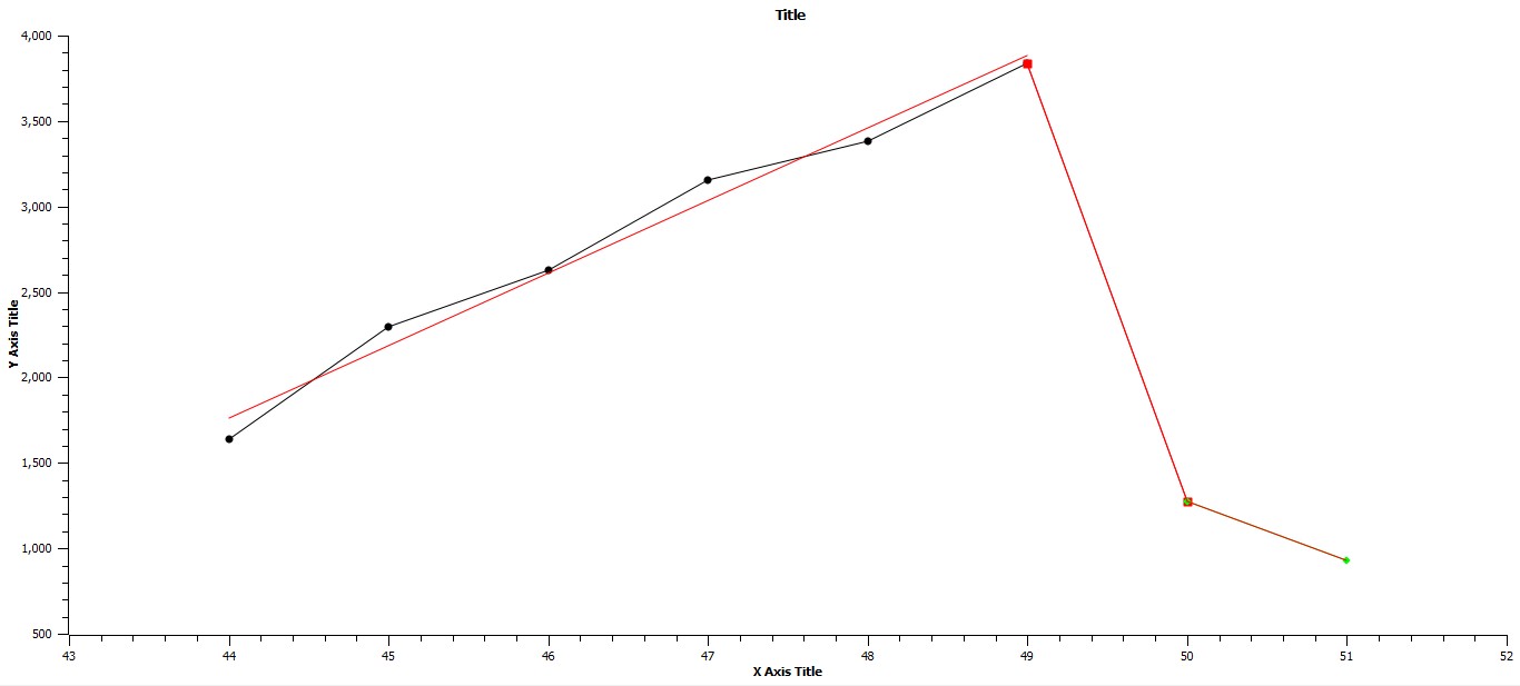
Fig. 10. Axes as in Fig. 7 but over the time span, 1400 CE to 2000 CE. The linear regressions for succeeding periods, 1400 CE to 1800 CE, 1800 CE to 1900 CE, and 1900 CE to 2000 CE are respectively: Y = 423.1254X – 16,852.8231 R² = .9844, Y = –2563.411X – 129,446.947 R² = 1, and Y = –347.759X + 18,644.347 R² = 1

One further point, in Fig. 11 to follow a graph of the ratio of maximum urban area magnitude to total world system population is given. Note that the four lowest points, all equal to or less than .0014, a value that appears to be a threshold point for system tipping. Three of these minimum values coincide with the beginning of each of the three periods of punctuation. The significance of the first value, the one not coincident with the beginning of a phase of punctuation, will be treated in the discussion.

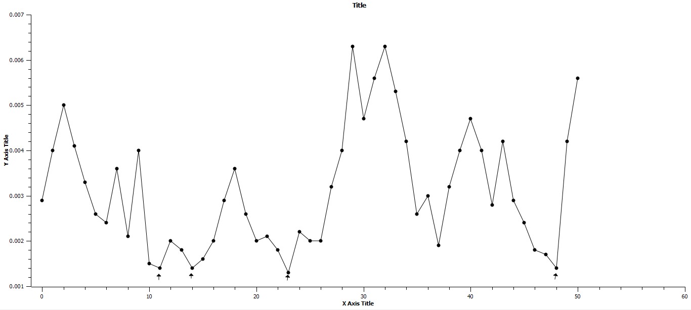
Fig. 11. The X-axis represents time in intervals of one hundred years and begins at 3000 BCE. The Y-axis represents the ration, C_max/T, where T = total population. Note the four arrows representing minimum values for this ratio. The timing of three of these low values coincides with the beginning of a phase of punctuation

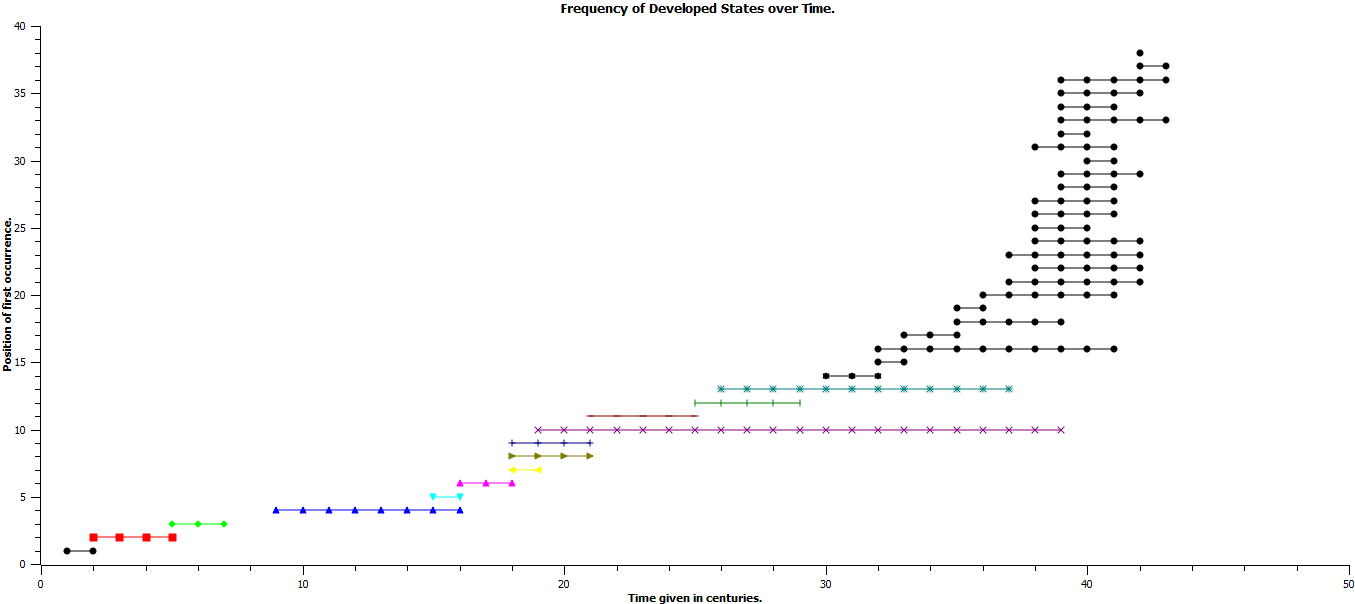
Fig. 12. The x-axis represents time in century increments beginning with Ur III, 2111 BCE and extending to 1900 CE. The y-axis represents the chronological order of first occurrence of the developed states represented in Table 1 of Grinin and Korotayev (2006)

Fig. 12 is introduced in concert with Figs 5, 9, and 10. Grinin and Korotayev (2006) suggest that developed states could not arise until a significant number of early states had formed and analogously the same holds true for the origin of mature states, i.e. that the existence of a significant number of developed states would be required prior to the advent of mature statehood. It can be seen that the frequency of developed states increases dramatically in the last seven centuries. This is illustrated more clearly in Figs 13a and 13b. In Fig. 13a there is a clear increase in the frequency of existent developed states from 1300 CE (note the arrow at 1300 CE) to 1800 CE with a significant decrease in the frequency of developed states in 1900 CE. If the accumulation of developed state-centuries is graphed against time as in Figure 13b, the graph appears sigmoid and the fourteenth century, again noted by an arrow, is at the beginning of this accelerated phase. All three of these graphs, Figs 12, 13a, and 13b, indicate a marked increase in the frequency of extant developed states and at a time over which the Industrial Revolution occurred, a time leading to and overlapping with the origin of mature states.

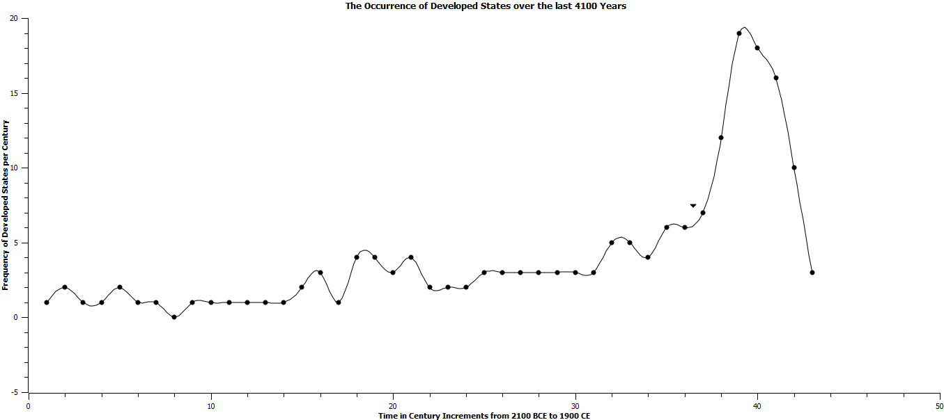
Fig. 13A. The occurrence of developed states over the last 4100 years

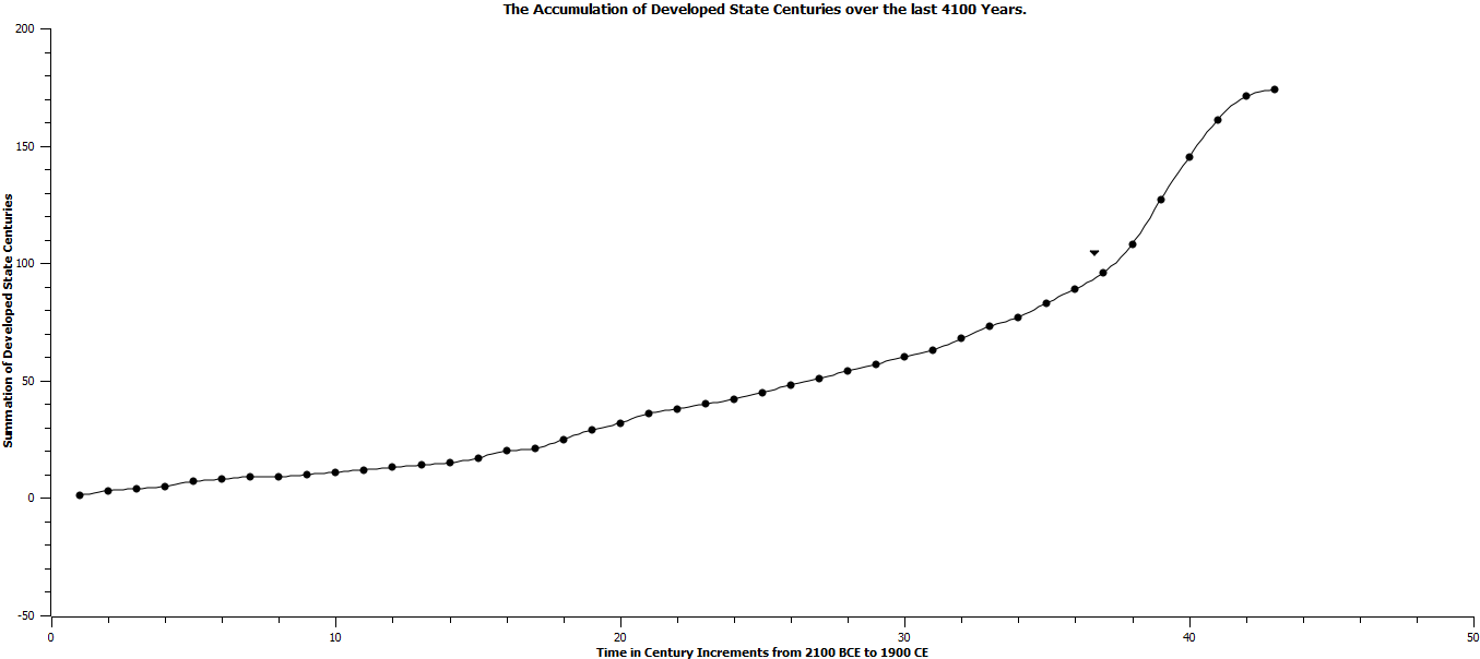
Fig. 13B. The accumulation of developed states centuries over the last 4100 years

A PRELIMINARY MATH MODEL OF PUNCTUATED GROWTH

An intuitively constructed mathematical model of punctuated growth is presented here, a model that is only a step above a reasonably well organized verbal metaphor, but such mental constructs do have their utility, as I hope will be seen shortly. Over fifty years ago Richard Levins (1968) suggested that there are three conditions affecting the functional nature of math models: generality, precision, and reality, only two of which would be operational at any given time for a specific model. The model presented here is general and precise; however, its ability to reflect the reality of punctuated growth for any given system is limited, and in fact may well be non-existent. The precision of this model is in my opinion only significant in that explicit values of a variety of variable can be predicted, but as was mentioned, those values do not have reality. Even so, having a general model has its heuristic value. One more comment here, a caveat, this model was specifically constructed to investigate the interplay between population, carrying capacity, and technology and makes no distinction between the world system population as a whole and the ever growing segment of that population dwelling in urban environments.

The model will be described first, data generated by the model will be presented, and then an explanation of the significance of the model will follow in the Discussion. To follow are the four differential equations of the model with supplementary equations and definitions of all constants:

dN₁/dt = r₁N₁[K – (N₁ + N₂)], dN₂/dt = r₂N₂[K – (N₁ + N₂)], dK/dt = [T – (N₁ + N₂)]/K, dT/dt = T/[K – (N₁ + N₂)], where N = population size, K = carrying capacity, r₁ = r₀₁ + aN₂, r₂ = r₀₂ + + bN₁, T = level of technology, and a and b as well as r₀₁ and r₀₂ are fitted constants. Initial and constant values: N₁ = 1.5, N₂ = 1, K = 5, T = 2, a = .016, b = .011, r₀₁ = .015, r₀₂ = .02, dt = .1.

Even at this level of relative model simplicity, the math modelling software, STELLA, had to be used to generate the following graphs. The model includes two interacting populations that exhibit positive feedback. This portion of the model was presented in Harper (2016) and is meant to show that population interaction of this nature leads to the form of growth identified by Korotayev et al. (2006) as hyperbolic. This effect is produced by the structure of the rates of growth of both populations, that is r₁ = r₀₁ + aN₂ and r₂ = r₀₂ + bN₁. These equations represent the condition that while each population has its base rate, either r₀₁ or r₀₂, the growth rate of each is enhanced by and dependent upon the other population. This dependency is represented by the terms, aN₂ and bN₁, where the constants, a and b, are greater than zero in value and represent the contribution of each population to the other's growth rate. However, complex systems, and the world system is nothing if it is not complex, have their limits.

Symbolic representation of limited population growth was first developed by Verhulst, and the same form of that representation, K – N, is used here. Specifically, the hyperbolic nature of these first two equations is limited by the term, K – (N₁ + N₂), implying that the two interacting populations occupy and exploit the same environment. Also however, the two populations can improve their environments, thus increasing the carrying capacity of the environment they both share. This environmental improvement is brought about by the use of appropriate technology. Consequently, that environment is subject to change, and in this model is represented by the third differential equation, dK/dt = [T – (N₁ + N₂)]/K, in which it can be seen that as the total population grows with respect to a given level of technology, the rate of change of the environmental carrying capacity decreases. As a result, the fourth equation in the model supplies a simple model of technological change in relationship to both population growth and change in carrying capacity. That equation is: dT/dt = T/[K – (N₁ + N₂)], and its structure is such that as the carrying capacity of the total population is approached, technological improvement, here represented simply by the quantitative change of the variable, T, is increased. The results of a simulation with the constant and initial values given above, is shown in the following graph which is a result of the simulation running over twenty-seven iterations:

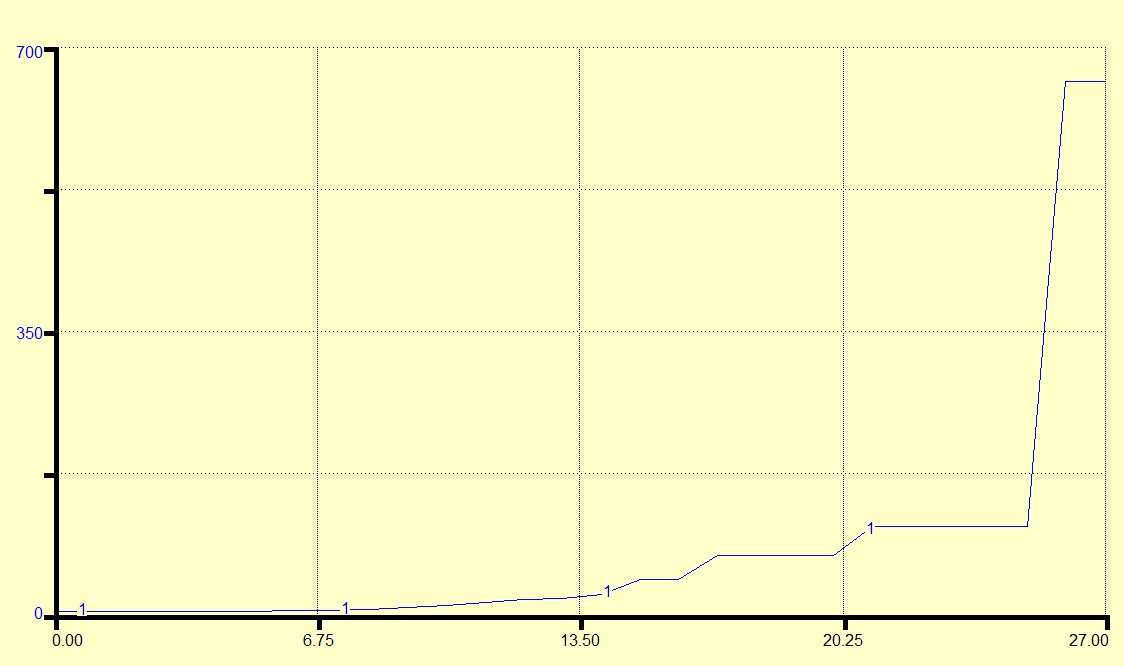
Fig. 14. The X-axis represents time in undefined units, and the Y-axis represents the magnitude of the total populations of both N₁ and N₂. The stepwise nature of the graph is clearly evident

It is evident that this graph, while representing population increase over time, does not represent continuous population growth but is characteristic of the structure of the graphs in Figs 2b, 3, 4, and 5. If the growths of both the carrying capacity and technology are represented over the same periods of time, the result appears as follows:

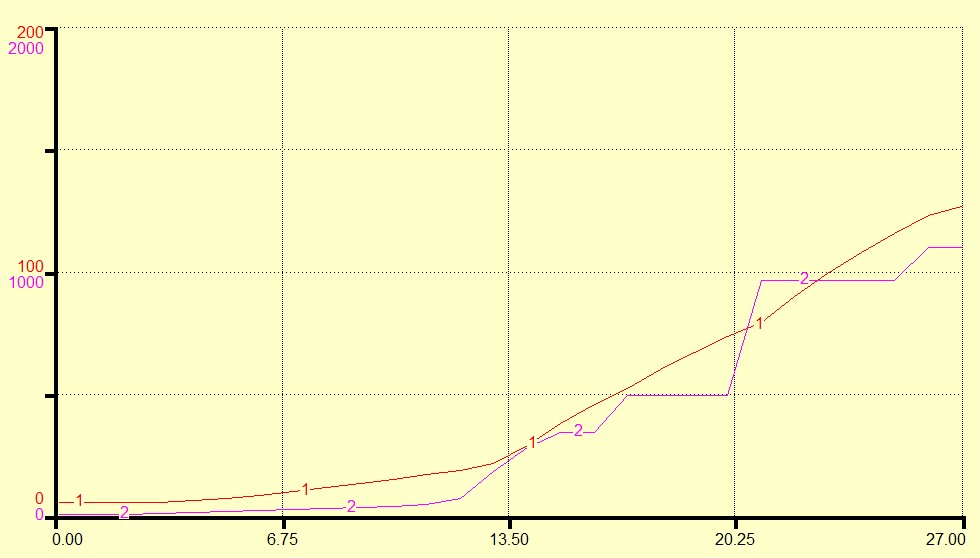
Fig. 15. The X-axis represents time in unspecified units, and the Y-axis represents the magnitudes of both carrying capacity, Kay, and technology, again in unspecified units

It can be seen that while the growth of technology is punctuated, the growth of the system carrying capacity is smooth(er) but with changing slopes indicating changing rates, but not of a punctuated nature. But if population size and the magnitude of technology are graphed as in Fig. 16 it can be seen that both seem to change in a similar fashion, although population change in this graph does not follow change in technology as suggested by Grinin and Korotayev (2006). This may be due to the resolution of the model, where dt = 1. The nature of these three graphs and their significance will be treated in the Discussion.

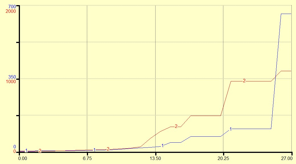
Fig. 16. The X-axis represents time in unspecified units, and the Y-axis represents the magnitudes of both technological developments and total population size, also in unspecified units. The designation, Enn, represents (urban) population size

The nature of these three graphs and their significance will be treated in the Discussion.

DISCUSSION

Preliminary to the discussion of the data introduced here, an elaboration of the previously introduced phenomenon of aromorphosis is necessary, as this is, as punctuated equilibrium is, one more model borrowed from the biological sciences to elucidate the mechanism of given social science processes. Specifically, aromorphosis provides as model for change in level of organization of, in the case of this paper, a form of social order, that of urbanization. The substance of what follows is taken from Grinin, Markov, and Korotayev (2009).

If one considers Figures 2b, 3, 4, and 5, the punctuated phases of change associated with the growth of urbanization are clearly represented, and in Fig. 2b specifically clear changes in the order of magnitude of maximum urban area can be seen, e.g. from populations of 100,000 to 1,000,000 during the period from 2100 BCE to 100 BCE, some 2000 years but in which the actual changes in order of magnitude occur over much shorter times, approximately half that time, specifically from 1600 BCE to 1200 BCE and from 700 BCE to 100 BCE. It is these periods of relatively rapid change for which aromophosis is being invoked.

Grinin, Markov, and Korotayev suggest rules for the occurrence of aroporphosis. Specifically, they suggest four necessary and sufficient conditions in order for arophophosis to occur. First, the system about to undergo aromorphosis must exhibit enough diversity. This is required for the establishment of positive feedback between different segments of the system. [Note here that positive feedback underlays the rapidity with which an aromorphic change may occur.] In any evolutionary process for change to occur selection must occur, and for selection to occur there must be something to select. With regard to the actual process, block assemblage is one way in which an aromorphic jump may occur, however, there must be a diversity of blocks from which to choose. This is their second rule. The third rule suggests that there is a direct connection, a direct proportional relationship between diversity and innovation. The fourth rule requires that there be efficient selection mechanisms leading to intergroup competition.

There are a variety of consequences to be noted for aromorphic processes. First, since selection occurs, there will be loss; selection always incurs a cost. Second, aromorphic change permits new adaptive zones to be exploited. Just as the evolution of the mammalian level or organization opened a variety of new adaptive zones and in a sometimes delayed fashion, that is mammals originating in the Triassic but only beginning their radiation in the early Cenozoic, for example, shrews, primates, hominins, the consequences of social aromorphosis may be delayed. Grinin, Markov, and Korotayev give the example of iron metallurgy originating at a period of time well before its spread after the (so called) Bronze Age Collapse. Third, aromorphosis enhances system resilience, since multiple functions can occur at the newly evolved level of organization that could not exist previously. Fourth, as just alluded to, multiple (new) functions imply increased complexity, and, fifth, with this newly acquired complexity new evolutionary changes can occur. Finally, aromorphosis permits previous limitations to the system to be exceeded. In fact, this is at the basis for the evolution of a new and higher level of organization to begin with.

The data of this study reveal two broad conclusions, that the summed pattern of change in maximum urban area population is similar to the pattern of punctuated equilibrium for speciation proposed by Eldridge and Gould and that the stasis phases are relatively different from the phases that represent punctuation. In fact, the pattern is more broadly speaking one of stasis punctuated by phase changes or phase transitions to further states of stasis. There are then at least three issues to be addressed, first, to confirm the punctuated nature of the evolution of maximum urban areas and its implication for the pattern of urbanization in general, second, to identify cues for the change from stasis to punctuation and the return to stasis, and, third, to suggest some form of mechanism for these changes.

The pattern of punctuated growth in urbanization has been alluded to by the following authors, Korotayev (2006), Grinin and Korotayev (2006), and Korotayev and Grinin (2006) and a mechanism mirroring punctuated growth has been proposed by Grinin, Markov, and Korotayev (2009). Regarding the dynamics of urbanization over time Korotayev has shown that while the overall pattern of urbanization is quadratic hyperbolic, because of the multiple agents operating within the world system over time, but largely mediated by feedback between population growth and the growth of technology intertwined with the accumulation of per capita surplus, the pattern of urbanization over time is not monotonic, that is smooth and continuous, but rather consists of periods of (relative) stasis punctuated by periods of more rapid growth. Review of Diagrams 7, 8, 9, 10, and 11 in Korotayev (2006) will confirm this. Also, in this paper Korotayev divides the periods of urbanization into sets A, one through three, and B, one through three, corresponding to periods of rapid growth, the A set, and cyclical change, the B set.

In tandem with this paper are two papers by Grinin and Korotayev (2006) and Korotayev and Grinin (2006) in which the specifics of political development both from the perspective of a quantitative analysis, the former reference, and a comparative analysis, the latter analysis, are given. In the first reference it is shown that the evolution of early, developed, and mature states corresponds to the periods of relative stasis, with the periods of punctuation being inserted in between each of these periods. In particular, the authors suggest that developed states are not possible until a significant number of early states exist, with the same holding for the existence of mature states, the implication that urbanization itself created the environment for further urbanization. It is interesting that this verbal model suggests a threshold or tipping point has to be breached before the next level of both urbanization and state evolution could occur, also supporting the position of this paper. However, as will be seen further on these tipping points can be exceeded in differing fashions depending on the context of the level of development (and complexity) of the world system. As will be seen shortly, this has particular pertinence with respect to the degree of fit to the linear regressions applied to both punctuated and especially stasis phases of urbanization.

As was noted in the initial portion of the Results section, in broad terms, the pattern of both population increase and maximum urban area increase is quite similar, and a very good linear fit of one set of log-transformed data against the other occurs with R² = .9179. However, as was also mentioned previously, on only slightly closer inspection, the pattern of urban area increase is quite different in detail. Specifically, there are three periods of stasis punctuated by three periods of rapid change, and these periods of rapid change are qualitatively different not only with respect to the rate of continuous change noted but also with respect to the variability of these periods of punctuation. These periods of punctuation are from 1600 BCE to 1200 BCE, from 700 BCE to 100 BCE, and from 1800 CE to 2000 CE, and linear regressions of the data of the three phases explain respectively 98.58 per cent, 97.32 per cent, and 99.98 per cent of the variability exhibited in each set of data. With respect to the three periods of stasis, from 2900 BCE to 1600 BCE, from 1200 BCE to 700 BCE, and from 100 BCE to 1800 CE, and their respective linear regressions explain respectively, .6 per cent, 37.59 per cent, and 13.02 per cent of the variability. Clearly, during periods of stasis there is much greater variability, a fact that seems incongruous with respect to the term, stasis. The point of course here is that these respective phases of the summed values of log-transformed values of maximum urban area magnitude are different both quantitatively and qualitatively. With regard then to the functional classification of state levels of evolution described by Grinin and Korotayev (2006), phases of stasis represent continuous adaptation of the world system at any given level of state organization, a process that will lead ultimately to movement to the next higher level of state organization. If these phase changes from punctuation to stasis and from stasis to punctuation are considered at a slightly finer scale, it can be inferred that interaction between differing segments of the total world system population are associated with these phase changes.

Regarding the surficial contradiction of the nature of the periods of stasis with respect to their variability, one has only to consider the slopes of their linear regressions to see that the variability represents oscillations about a mean for periods of stasis. Specifically, the slopes of the periods of stasis are all close to zero or horizontal, that is –.0064, –.0573, and .0198. This plateau-like nature of these periods has been noted before (Harper 2010; Korotayev 2006; Grinin and Korotayev 2006; Korotayev and Grinin 2006), and in slightly different form have been noted by Morris (2013). He specifically suggests that there have been plateaus with respect to maximum urban area magnitude of ten thousand, one hundred thousand, and one million, and twenty-five million, and while I would use slightly different values of forty-thousand, one hundred thousand, one million, and most recently something above thirty-five million, given the margin of error in the proxy data used, the notion of stabilizing values of maximum urban area magnitude existing over periods of time is in agreement with the data at hand.

It is interesting that the interaction between rural and urban populations seems to play a major role in the establishment of periods of stasis and punctuation in the macropattern of urbanization. During periods of stasis the average maximum size of urban areas remains static but gamma, basically the variable indicating the distribution of urban areas as defined by a Zipf-Pareto distribution, increases implying that greater urbanization is occurring at urban area sizes below that of maximum. In other words, as the total population of the world system increases, even though the top end of the distribution of urban areas remains relatively constant, the total urbanized population can potentially increase due to the expanded sizes of sub-maximal urban areas. If one calculates the size of sub-maximal urban area populations while holding the maximum urban area population constant and allowing gamma to increase, the sizes themselves increase, and this is in fact the pattern seen from the fourteenth century to the beginning of the nineteenth century. During this period of time maximum urban area size remained essentially constant at approximately one million or slightly more, and yet the total population of the world system increased from 350 million to 813 million and gamma increased from 1.3483 to 1.4112, a clear indication of increasing urban area size below maximum. Further, the increase in population was accommodated in a predictable way a la a Zipf-Pareto distribution. This effect is alluded to in both Diagrams 1 and 5 of Korotayev and Grinin (2006) in which the territory of developed states increased at a greater rate than did the urbanized population of the world system over essentially that same period of time. What is also implied here is that movement from the rural population to urban areas, more so than the birth rate endemic to urban areas simply because the death rate characteristic of urban areas is higher than that of rural areas and also very often is higher that urban birth rates, is responsible for this growth in urban population. Further, with regard to the level of evolved state, early, developed, or mature, the change from a lower level of state to a higher level requires that urbanization precede the change. In fact, it is this increase in urbanization, especially at maximum size that contributes to the change from early to developed state and then from developed to mature state. However, phases of stasis may well involve increase in urbanization at lower levels of urban area size. Increase in urbanization does not always occur simply by dint of movement.

As previously implied this is unquestionably not the end of the process, as technology plays a significant role in the evolution of both urbanization and level of state development. Korotayev and Grinin (2006) make the point that technology leads the process of urbanization and improvements, new evolved levels of technology, must occur prior to any increase in urbanization. They use a particularly effective example of the advent and spread of iron technology, suggested by them to initially originate with the Hittites. However, on collapse of the Bronze Age (at the eastern end of the Mediterranean) and due to the attendant collapse of extensive trade routes at that time the production of bronze implements of war and peace, that is agriculture, was not possible. Instead, iron technology was adopted due to the relatively easy access of iron. This technology required time to spread, so, since the evolution of urbanization follows the evolution of technology, urbanization at this time was delayed as was the evolution of the developed state.

A further point needs to be made here and is dependent on the work of Per Bak (1996) and of Flyberg et al. (1993). These researchers have shown using a simple computer model of evolution that evolving systems self-organize in a punctuated fashion up to a critical point, a point which Bak labeled as the state of self-organized criticality (SOC). Further, the research of Bak, Flyberg, and others has demonstrated that the stepwise changes are due to changes in maximum fitness, with variability in the system being due to the range of fitnesses, which when minimum fitnesses are eliminated push the system to the next higher level. While I am not in the position of fitting such model expectations, the data at hand do fit the pattern of punctuated change and similarity of appearance is suggestive, that is if it looks like a duck, quacks like a duck, flies like a duck, and so forth, it is probably a duck. Unquestionably however, there is potential fallibility in this reasoning, since the duck in question could also in reality be a goose. Even so, I am invoking the reasoning of Bak et al., as they present a model consistent with the data at hand in that as a consequence one would expect fluctuations above (or about) some minimum or median value of stasis until a cue occurs for the system to move to the next higher level, and this is what the data here on the summed values of natural log-transformed magnitudes of maximum urban area reveal. [Parenthetically, I would like to mention that this research assumes that the world system has not reached the ultimate state of self-organized criticality but quite clearly appears to be headed in a direction that will lead at least to a level of self-organized criticality limited by the degree of urbanization and state organization, as any self-organizing system would unless of course collapse of some magnitude ensues.]

In summary, the data presented in this paper, the data presented by Morris (2013), by Grinin and Korotayev (2006), Korotayev (2006), by Bak (1996) and by Flyberg et al. (1993) either support the notion of stasis in the macropattern of urbanization, that is the existence of some limiting mean about which oscillation occurs, or provide an underlying mechanism for the existence of such a mean. It should be noted that saltation from one stasis mean to the next requires an increase in either energy sources available or the technology to more efficiently exploit already available resources. This in turn supports the concept presented by Grinin and Korotayev (2006) that, as was mentioned previously, technological improvement precedes the development of urbanization to the next level. It should further be noted that the process being explained fits well with the concept of aromorphosis introduced at the beginning of this discussion (Grinin, Markov, and Korotayev 2009). That the narrative of human history should no longer be considered a sequence of individual events per se, at least at the macro-scale, and that there is a clear evidence for punctuated change in human history at least as it is reflected in the evolution of urbanization and also for the existence of logico-deductive models to explain that mode of change should now be clear. What follows, even if somewhat repetitious, supports this notion.

If Fig. 1a is inspected and compared with Fig. 2b, there is clear agreement with respect to overall form, but Fig. 2b shows clearer distinction between periods of stasis and periods of punctuation. It is for this reason that the summed values of changes in the natural log-transformed maximum urban area size were used. Also, to reaffirm, a graph of the individual values of the urban area data would not on inspection reveal any significant difference between periods of stasis and those of punctuation. Given the step-wise appearance of Fig. 2b, what is implied by its form? First, it is apparent that history at the level of maximum urban area evolution, and therefore urban area evolution in general and based on the assumption of urban areas being distributed in a Pareto-like fashion, has not simply been ‘one damned thing after another’ (Toynbee 1976), but that there have been distinct periods or phases of history, each representing different modes of change. Again, the mechanism for these differing modes of change fit very clearly with the concept of social aromorphosis as developed by Grinin, Markov, and Korotayev (2009) and with the very general model of punctuated change in biological evolution as presented by Flyberg, Sneppen, and Bak (1993). Although, the combinations of stasis and punctuation do repeat, so, perhaps Toynbee should have said that history ‘is just one stasis phase followed by one phase of punctuation after another.’ On the one hand, periods of stasis represent fluctuations about some mean maximum urban area value of change or above some minimum threshold of the same a la Bak. On the other hand, phases or periods of punctuation represent movement of the world system as represented by maximum urban area change to new and higher levels of stasis. These two distinct phases have associated with them distinctly different ranges of variation as mentioned previously, stasis with exceptionally low values and punctuation with exceptionally high values. The implication of the former, I believe, suggests some form of system searching, while the latter suggests some relatively rapid change, perhaps very closely canalized or perhaps of an autocatalytic fashion that occurs so (relatively) quickly that the system itself is responding in an exponential or hyperbolic way. A brief discussion of the following time periods, 2900 BCE to 1200 BCE, 1200 BCE to 100 BCE, and 100 BCE to 2000 CE will follow. Each of these periods represents a combination of an initial period of stasis followed by a period of punctuation.

The period from 2900 BCE to 1200 BCE is the most problematic, as it exhibits several sequential fluctuations, only one of which is identified here as associated with a period of punctuation, the last and smallest fluctuation (see Fig. 3). The R² value for the stasis phase of this period, .0060, is very low, confirming that the range of data, that is the fluctuation exhibited by the data, is considerable. All other fluctuations during this period are associated, I believe, with the initial establishment of empire and how that initial establishment induced its own ecological overshoot as described in the book of the same name (Catton 1983) and as a result do not fit the criteria established for a phase of punctuation. (Parenthetically, aromorphosis must play a significant role directly in the initial establishment of empires, for example, the Akkadian and Ur III empires, but this appears not to be associated with a change in the level of urbanization, as urbanization should precede such territorial extension. However, such events in relation to energy acquisition are worthy of future research.) Note, for instance, that the period from 2100 BCE to 2000 BCE represents a decline in the Akkadian Empire and is also associated with very harsh climatic changes. The actual punctuation phase begins at 1600 BCE and follows a decrease in summed change from the previous century, in fact this point at which the punctuation begins represents the regressed mean value of the previous period of stasis as can be seen from the graph. The beginning of this phase is a point shared by both initial stasis and the following phase of punctuation. Interestingly, this pattern is consistent with the change from stasis to punctuation in the remaining two time periods as well. Of note here also is the fact that the ratio of maximum urban area value over the total population of the world system is at or less than .0014, a threshold minimum that holds for similar points in the other two periods. Why this particular minimum should hold is not clear.

In the second combined period of stasis and punctuation, from 1200 BCE to 100 BCE, a change from stasis to punctuation at 700 BCE is exhibited, and this occurs a century after the (approximate) beginning of the Axial Age as established by Karl Jaspers (1953). The stasis before this point in time has R² = .3759, implying that the range of fluctuation was considerably lower than that of the previous stasis phase, while that of the phase of punctuation to follow is R² = .9732, which is consistent with the R² values for the other two phases of punctuation. It is also interesting here that the stasis phase is shorter than the phase of punctuation, five hundred years as opposed to six hundred years, not inconsistent with the data of Bak but intuitively surprising in light of the length of the stasis phase of the previous period investigated. This period of lengthy punctuation reaches a regressed mean of one million for the size of the maximum urban area in the next stasis phase and spans the time when the first quasi-global empires were established, the Han Empire and the Roman Empire. Trade also became essentially global at that time with the establishment of the Silk Road and the water routes of the Mediterranean Sea, Indian Ocean, and points east into Indonesia and along the eastern coast of China. As will be seen, this level of complexity required a considerable period of search time before cuing the next phase of punctuation. In more quantitative terms, the system search achieved low ratios for C_max/T ≤ .0014 twice during this period of 2100 years, only one of which is associated with the phase of punctuated growth that we are now in.

The third and final period to be considered extends from 100 BCE to 2000 CE, is the longest of the three periods, and is the one we are all currently living in. The phase of stasis associated with period of twenty-one hundred years is the longest of the three phases investigated, and involves three peaks, two troughs, and a four hundred year period of actual stasis with little fluctuation in maximum urban area magnitude before entering the final period of punctuation. This period of time spans the apogees of the Han and Rome empires, the European Dark Ages, two monumentally significant plagues, Justinian's and the Black Death, the European Renaissance, the Age of Discovery, the evolution of democracies, and the list goes on and on, and with a variance value of R² = .1302 is clearly a period of time when the distribution of points, of the change in maximum urban area magnitude, varies considerably about a linearly regressed mean. This is then a period of system's search before entering the current period of punctuated growth and represents an extended period of time over which new technologies affecting both the discovery of new energy sources, that is the fossil fuel triad of coal, oil, and gas, were not accessed in any substantial way until the middle of the eighteenth century CE. In turn, the three points of the current period of punctuation extending from 1800 CE to 2000 CE and into the current time have a variance value of R² = .9998. This is a period of time in which the end phase of the Industrial Revolution (Grinin and Korotayev 2015) propelled the world into the Industrial Age followed by the post-Industrial Age, a time when the size of the maximum urban area increased from 1.1 million in 1800 CE to the megacity of Tokyo, which currently is approximately hosting a population of thirty-five million, and a time in which the exponent, γ, a measure of urban distribution, decreases from γ = 1.4112 to 1.2099. The implication of this decrease is that there are now far more urban areas in which our population is housed than ever before, and consequently this last two hundred years has seen a massive movement of humanity from a largely rural existence to a largely urban one.

As mentioned previously, this interplay between rural and urban populations, one currently shifting the balance in favor of urban occupation to the extent of 70 per cent of the world system population by 2050 has of course been going on since the Neolithic Revolution. What the previous portion of this discussion suggests is that new levels of urbanization have been achieved in a step-wise fashion, and that, further, this occurs against a demographic backdrop of more of less continuous increase in world system population. The relationship between the population as a whole and the process of urbanization will be addressed next.

As can clearly be seen from Fig. 1, both the total population of the world system and the magnitude of maximum urban area show similar patterns of development over the last five thousand years, however, as has been already addressed, the detail of these patterns differs with the development of total population exhibiting a smoother pattern over all, while maximum urban area magnitude both increases and decreases against the background of more or less steady population change. Further, the exponent, γ, which characterizes the pattern of urbanization per time point and is predicated on the distribution of urban areas being Pareto-Zipf-like, also changes in a fluctuating pattern, in fact the mirror image of that of urban areas. It is particularly interesting to note that per stasis phase, the total population increases, while at the end point of each phase, the final value of maximum urban area magnitude is at the regression mean. In other words, while total population increases, and one would intuitively expect that maximum urban area magnitude would also, in the final point of that phase, one shared with the succeeding phase of punctuation, the maximum urban area value is exactly at the regressed mean. However, at the same time, the value of γ is maximum for the phase. What does this imply? It implies, I believe, that the increased population is housed in a greater abundance of lower level urban areas and that populations that were essentially not urbanized at the beginning of a give phase of stasis now are.

The event of stasis is then characterized by the following process: After a period of continuous maximum urban area increase and against a background of more or less continuous total population change, over the period of time associated with stasis, the increased total population is then housed in more urban areas of smaller scale. The process of stasis, of accommodating greater total population with in a framework of both urban and rural environments, is done so also against a stable maximum urban area magnitude and exhibits fluctuations about this stable maximum until the final fluctuation achieves some tipping point at which maximum urban area magnitude increases for an extended period of time. Each upward movement of the system during stasis, that is each increase in maximum urban area magnitude with its attendant change in the frequency of lesser urban areas, can be thought of as an attempt to challenge the upper limit of the system set by the maximum urban area magnitude of that stasis period.

There are also minimum sizes with respect to the regressed mean of any given stasis phase which seem to be roughly the regressed mean of the previous stasis phase. However, when the ratio of maximum urban area magnitude to total world system population is calculated, there appears to be a threshold minimum value at and below which is initiated the next phase of punctuation. That value is .0014, and this represents another way of considering the context in which a phase of punctuation originates. There are four such points as represented in Fig. 11, the last three of which correspond to the initiation of phases of punctuation. The low value point does not represent such an initiation and is probably a consequence of external factors; climatic factors are the most obvious candidate. It is proposed, then, that some sort of cue or trigger exists in which rapid, continuous urbanization follows from one stasis level to the next and as previously mentioned is controlled by a tipping point.

Tipping points are points in a process in which the process itself changes rapidly. They may be thought of as phase changes, and there are broadly two types of tipping points, direct and indirect (Lamberson and Page 2012). Direct tips are those in which a continuous increase in a given data set produces at some point a rapid increase in that same data set, while an indirect tip is one in which continuous change in one type of input causes a rapid change in a different type of output. An example of the former is, and an example of the latter is a diabetic slipping into a coma due to low blood sugar. Also, tips can be characterized by changes in either entropy or diversity before and after the point of tipping. In the case of entropy, the Shannon-Weaver index is used, H = –∑plnp, where p is the frequency of some entity, while changes in diversity can be monitored by the formula: D = ∑1/p². The second formula is used here.

Figs 7, 8, and 9 represent graphs of the tips associated with the phases of punctuation from 1200 BCE to 100 BCE, from 3000 BCE to 1200 BCE, and from 100 BCE to 2000 CE. These graphs were listed out of chronological order, as the graph of change from 1200 BCE to 100 BCE was thought to be the most characteristic of tipping and was therefore presented first as a model against which the other two graphs could be compared. The tipping points themselves in each of these time periods fall between 700 BCE and 600 BCE, 1800 BCE and 1700 BCE, and between 1800 CE and 1900 CE respectively. In each case the tip occurs after the actual punctuation phase begins. Why should this be?

It is proposed here that the system continually fluctuates/oscillates around a stasis level the ceiling of which is continually tested. In this context then it is easy to understand that over time the testing of the ceiling of each stasis period will produce increasing sub-phases only the last of which will induce punctuation. As a consequence of this, a tip to initiate punctuation would be expected to occur after the actual punctuation phase had begun.

Any proposal of mechanism at the present point of this research must be put in the category of speculation, and so what follows is exactly that. However, it is hoped that by presenting such a proposal thought will be stimulated to consider ways of testing the proposed mechanism or perhaps even addressing the problem, that of what causes the occurrence of tipping points and their attendant phases of punctuation, from an entirely different context. Given this preamble, what follows is a mechanism consistent with the data used.

First, it should be noted that in general terms a mechanism already exists, that of Flyberg et al. (1993) in which an evolving system moves to a position above a minimum selective threshold and then proceeds to test the upper boundaries of the selective environment until a new and higher minimum is achieved. The explicit problem that I see here is how this general notion can be matched to the specifics of the urban-rural dance that occurs during stasis to ultimately reach a tipping point. During phases of stasis diversity exhibits a general trend of increase, and as part of the mechanism to generate a tipping point it is proposed that this is a necessary condition. However, while increased diversity is necessary, it is not sufficient, because diversity, and here diversity is meant as a proxy for specialization, does not imply linkage within the system. It simply refers to the differentiation of parts within the system. The linkages that are necessary really imply the establishment of positive feedback which will bring about the necessary urban growth to institute a phase of punctuation. In turn, positive feedback is a consequence of establishing hypercycles, the entity proposed by Eigen and Schuster (1977) to exceed the limitations of the reproductive (and information) paradox that he discovered and now bears his name. The question then is: What process establishes (a) hypercycle(s) which in turn create(s) the positive feedback to further create a punctuated phase of urban growth? [For a simple and lucid explanation of what hypercycles are all about, see Smith and Szathmary (1995), Chapter 4 The Evolution of Templates, Section 4.5 The Hypercycle.]

To answer this question the work of Padgett et al. in Padgett and Powell (2012) will be cited. Specifically the work of Padgett and others is focused on how organizations and markets emerge from a milieu, an environment, of firms, skills, and exchanges. They suggest that such emergence is autocatalytic, the result of which is the development of one or more hypercycles and give a detailed explanation of emergence and probability of survival under a variety of conditions, for example, a depauperate environment, an enriched environment, restricted emergence to a single hypercycle, and emergence involving the creation of multiple hypercycles. The model to be used here is simply a hypercycle involving two entities, a rural population with its attendant characteristics and an urban population with its own adaptive characteristics. These two components exchange goods and services and in doing so create a hypercycle that sustains both. It should be noted here that this relationship has been noted earlier (Harper 2016) and in that model the emergence of hyperbolic growth is represented. The specific assumptions and points of the current model are as follows:

1. The world system is a self-organizing system.

2. As previously asserted, the model of self-organization is that of a hypercycle.

3. Hypercycles are sets of interconnected components which feed off each other and supply each other with the essential resources for existence.

4. Hypercycles have limits with respect to their level of complexity and rate of function.

5. During periods of stasis the world system hypercycle(s) organize in order to make the next ‘jump’, that is to enter a phase of punctuation.

6. In order to do this, diversity of components is maximized.

7. A punctuation phase then ensues with its attendant loss of diversity and stops at the next (proximal) limit.

8. Stasis begins again and diversity expands, albeit in a nonlinear and fluctuating fashion.

This verbal model can also be complimented by very general mathematics.

A preliminary math model of punctuated growth was also presented, and the graphical data generated by this math model shows that a system operating with the explicit structure and constraints of the model exhibits punctuated growth. What is the implication of this type of growth for the world system? I believe that punctuated growth is an inherent part of the process of world system growth as reflected by urbanization and in fact at a very coarse level of simulation is due to the interactions between population, carrying capacity, and technology; the model certainly implies this. Fig. 14 shows a pattern of population growth not unlike that of world system population growth shown in any number of publications by Korotayev and Korotayev and colleagues, for example, Korotayev, Malkov, and Khaltourina (2006 a, b, and c) and is also similar to the patterns represented in Grinin and Korotayev (2006) and Korotayev and Grinin (2006). However, what is worth of a relatively simple model, a general model, of such system behavior?

There are several benefits of such a model; three will be given here. As at its present stage of development the model only reveals a general level of similarity with the data presented here and not explicitly matched values, its overall structure then is reminiscent of the general nature of such systems. The rapid change in population size is due to the hyperbolic nature of the growth of two interacting populations within the model. This is certainly in keeping with the pattern of world system population growth over the last five thousand years, the changes in urbanization level are, however, not continuous, also in keeping with world system behavior over the historical period, as are changes in technology. Of a more dubious nature is the pattern of carrying capacity change, which is not discontinuous but continuous with changing slopes associated with the punctuated changes in both population size and the level of technology. The model then suggests a mode of further research into the (more) explicit interactions between these three variables.

System size is also revelatory. The system represented by this math model is a small one, nothing like the level of complexity of the world system even though it exhibits some of the same behavior. Perhaps what is implied then is that the real system is either heavily buffered or that at different levels of organization processes at sublevels reach thresholds, tipping points, that cause response at higher levels. The process of social aromorphosis as detailed by Grinin, Markov, and Korotayev (2009) certainly would be consonant with such changes, and specifically associated with aromorphic changes would be changes in the level of evolution of the state.

Thirdly, the graphical system behavior suggests that thresholds are breached with respect to what the carrying capacity will allow, and the system as a whole responds very quickly due to the interaction of the two population system. Considering hypercycle formation as a motivation for aromorphic change then suggests that in the actual data for world system urbanization change the timing of such hypercycle formation must occur prior to punctuated change, and it is during these periods that evidence for such hypercycle formation should be searched for. While the periods of stasis as represented by the model do not exhibit fluctuations, it should be noted that such periods do exist over significant segments of model time, and this length of time is scaled to the punctuated change to follow.

The model in both its verbal and mathematical forms proposed above is barely a shadow of its future self, and clearly there is a sense of vast incompleteness. First, the model barely exceeds the level of a narrative description. Second, mechanisms let alone mechanisms within mechanisms have yet to be defined. For example, consider the following two questions: How is diversity actually maximized? What establishes hypercycle limits and rate of function? Third, and for the moment finally, a specific form of the simple two component hypercycle of rural-urban interaction has yet to be established, as has the analogue of Eigen's paradox with respect to the change in level of urbanization that the world system has exhibited over the last five thousand years of its history. However, even with this sense of ‘vast incompleteness’ identified, it is hoped that the proposed model will further thought and research on the mechanisms of punctuation and stasis that have characterized world system self-organization and therefore evolution over historic time.

SUMMARY

1. Change in complex systems is neither simple in occurrence nor in mechanism.

2. The phenomenon of punctuated equilibrium as first proposed and described by Eldridge and Gould has broader application than simply to the process of speciation and is common to a variety of Big History scenarios.

3. While it is understood that punctuated equilibrium falls within the domain of biology and is therefore a phenomenon best studied within the domain(s) of science, it is the position of this paper that history is a science.

4. The focus of this paper is the occurrence of punctuated equilibrium in the evolution of urbanization over the course of world system history, and world system analysis gives this paper its primary context.

5. The work of Per Bak and others is also used not only to add to the context of this study but also to provide a general mechanism for the process of punctuated equilibrium.

6. Natural log-transformed data for both maximum urban area magnitude and the magnitude of total world system population constitute the raw data for this study.

7. The summed data for maximum urban area magnitude was used, as it provided clearer evidence for the distinction between stasis and punctuation than did the unsummed data.

8. It is assumed that per increment of time urban areas have a Pareto/Zipf distribution.

9. There is clear similarity in pattern between the graphed data for maximum urban area and for total population over time. However, on close inspection, the data for maximum urban area reveals three phases of stasis separated by three phases of punctuation.

10. Punctuated patterns in world system change have been recognized previously with respect to urbanization, state evolution including state territory size, and the fact that state evolution has produced three different levels of organization, early, developed, and mature states which fit nicely with the pattern of punctuations and stasis investigated here.

11. Each type of phase is characterized by its own R² values. Those of phases of stasis are very low, implying great variation, and those of phases of punctuation are very high, implying that the process of punctuation is very directed.

12. The research of Leonid Grinin and Andrey Korotayev with respect to both the formal and comparative quantitative analysis change of urbanization over time and the work of Andrey Korotayev on urbanization dynamics have particular significance here.

13. A simple measure of diversity was used to identify the presence of tipping points from stasis to punctuation.

14. The existence of tipping points in the evolution of world system urbanization implies that continuous change in diversity is interrupted at key points as the system switches from mode of a stasis to a mode of punctuation.

15. Tipping points occur after the apparent initiation of punctuation due to the fact that during stasis the system fluctuates in urban area distribution as represented by γ, that is the system searches for the next higher level of urbanization.

16. Minimum values for the ratio, C_max/T ≤ .0014, occur four times in world system history, three of which are associated with the apparent initiation of a phase of punctuation.

17. The plateau-like nature of maximum urban area evolution has also been noted by Morris.

18. World system history at least as revealed here by the data on maximum urban area magnitude is not just an occurrence of events, one after another, that is historically contingent events with little overall context, but is on the contrary a process with structure. That structure is a consequence of phases of stasis alternating with phases of punctuation.

19. A mechanism is proposed in which it is assumed that the world system is a self-organizing system and uses as its mode of self-organization the hypercycle. Hypercycle evolution is tied to the gain (= stasis) and loss (= punctuation) of the diversity of urban area sizes.

20. The process of social aromorphosis is also evident as a contributing mechanism for punctuated change.

21. A simple math model of punctuated change was developed to show the general characteristics of that change as a result of the interaction between population, carrying capacity, and technology.

MATHEMATICAL APPENDIX

Determination of p-values for D = ∑p_m^-2.

Given that the distributions of urban areas can be given by the formula, F = αC^-γ, where F = frequency, α = C^γ, and γ = a fitted constant determined numerically from the equation, C_max^γ – C_max – – (γ – 1)T = 0 (see Harper 2010 for details of the derivation) and assuming that the actual sizes for urban areas follow a distribution of 2^m, where m = the index of urbanization, so that C_max = C_max2⁰, and urban areas having a frequency of 2 have m = 1, that is for the magnitude of C₁ = [C_max/2]^γ, and for m = 2, C₂ = [C_max/2²]^γ, and so forth, then to find the total urban population for each m simply multiple the previous formula by 2^m, that is C_max2^{m(1 – 1/γ)}. It is these values that are used for m = 0, 1, 2, and 3 that are used to determine the appropriate p-value for the computation of D = ∑p_m^–2 in the following way: 1. Compute C_m for m = 0, 1, 2, and 3. 2. Sum all values. 3. Divide each C_m by the total to compute each p-value. 4. Use the formula above to compute D.

REFERENCES

Bak, P. 1996. How Nature Works: The Science of Self-Organized Criticality. New York: Copernicus.

Catton, W. R. 1983. Overshoot: The Ecological Basis of Revolutionary Change. Chicago. University of Illinois Press.

Chandler, T. 1987. Four Thousand Years of Urban Growth: An Historical Census. Harvard: Edwin Mellin Press.

Eigen, M., and Schuster, P. 1977. The Hypercycle: A Principle of Natural Self-Organization. Part A: Emergence of the Hypercycle. Die Naturwissenschaften 64: 541–565. URL: http://jaguar.biologie.hu-berlin.de/~wolf ram/pages/seminar_theoretische_biologie_2007/literatur/schaber/Eigen1977Naturwissenschaften64.pdf.

Eldridge, N., and Gould, S. J. 1972. Punctuated Equilibrium: An Alternative to Phyletic Gradualism. In Schopf, T. J. M. (ed.), Models in Paleobiology. San Francisco: Freeman Cooper.

Frank, A. G., and Gills, B. 2014. World System: Five Hundred Years or Five Thousand. New York: Routledge.

Flyberg, H., Sneppen, K., and Bak, P. 1993. Mean Field Theory for a Simple Model of Evolution. Physical Review Letters 71: 4087.

Forester, H. von, Mora, P. M., and Amiot, L. W. 1960. Doomsday: Friday, November 13, A.D. 2026. Science 132: 1291–1295.

Grinin, L., and Korotayev, A. 2006. Political Development of the World System: A Formal Quantitative Analysis. In Turchin, P., Grinin, L. E., de Munck, V. C., and Korotayev, A. V. (eds.), History and Mathematics: Historical Dynamics and Development of Complex Societies (pp. 115–153). Moscow: KomKniga.

Grinin, L., Korotayev, A. 2015. Great Divergence and Great Convergence: A Global Perspective. Springer.

Grinin, L. E., Markov, A. V., and Korotayev, A. V. 2009. Aromorphosis in Biological and Social Evolution: Some General Rules for Biological and Social Forms of Macroevolution. Social Evolution and History 8 (2): 6–50.

Harper, T. 2010. The Trajectory of the World System over the Last 5000 Years of History. In Grinin, L., Herrmann, P., Korotayev, A., and Tausch, A. (eds.), History and Mathematics: Processes and Models of Global Dynamics (pp. 13–63). Volgograd: Uchitel.

Harper, T. 2015. A Toy Model Mechanism for Greater-Than-Exponential Human Population Growth. (In Press.)

Harper, T. 2016. Punctuated Equilibrium, a Pattern Common to Big History that also Characterizes the Pattern of Urbanization. (In Press.)

Jaspers, K. 1953. The Origin and Goal of History. New York: Routledge and Kegan Paul.

Korotayev, A. 2006. The World System Urbanization Dynamics: A Quantitative Analysis. In Turchin, P., Grinin, L., Korotayev, A., and de Munck, V. (eds.), History and Mathematics. Historical Dynamics and Development of Complex Societies (рр. 44–62). Moscow: KomKniga/URSS.

Korotayev, A., and Grinin, L. 2006. Urbanization and Political Development of the World System: A Comparative Quantitative Analysis. In Turchin, P., Grinin L., Korotayev A., and de 74 Globalistics and Globalization Studies Munck, V. (eds.), History and Mathematics. Historical Dynamics and Development of Complex Societies (рр. 115–153). Moscow: KomKniga/URSS.

Korotayev, A., Malkov, A., Khaltourina, D. 2006a. Introduction to Social Macrodynamics: Compact Macromodels of the World System Growth. Moscow: Editorial URSS.

Korotayev, A., Malkov, A., Khaltourina, D. 2006b. Introduction to Social Macrodynamics: Secular Cycles and Millennial Trends. Moscow: Editorial URSS.

Korotayev, A., Malkov, A., Khaltourina, D. 2006c. Introduction to Social Macrodynamics: Secular Cycles and Millennial Trends in Africa. Moscow: Editorial URSS.

Lamberson, P. J., and Page, S. 2012. Tipping Points. URL: http://www. santafe.edu/media/workingpapers/12-02-002.pdf.

Levins, R. 1968. Evolution in Сhanging Environments. Princeton: Princeton University Press.

Modelski, G. 2003. World Cities: –3000 to 2000. Washington, D.C.: FAROS 2000.

Morris, I. 2013. The Measure of Civilization: How Social Development Decides the Fate of Nations. Princeton: Princeton University Press.

Ortman, S. G., Cabaniss, A. H. F., and Bettencourt, L. M. A. 2013. Urban Scaling in Pre-Hispanic Mexico. SFI Working Papers. 2013-01-001 http://www.santafe.edu/media/workingpapers/13-01-001.pdf.

Ortman, S. G., Cabaniss, A. H. F., Sturm, J. O., and Bettencourt, L. M. A. 2014. The Pre-History of Urban Scaling. PLOS. http://journals.plos. org/plosone/article?id=10.1371/journal.pone.0087902.

Padgett, J. F., McMahan, P., and Xing Zhong 2012. The Emergence of Organizations and Markets. Princeton: Princeton University Press.

Scheffer, M. 2009. Critical Transitions in Nature and Society. Princeton: Princeton University Press.

Smith, J. M., and Szathmary, E. 1995. Major Transitions in Evolution. New York: Oxford University Press.

Sole, R. V. 2011. Phase Transitions. Princeton: Princeton University Press.

Toynbee, A. 1976. The Toynbee-Ikeda Dialogues: Man Himself Must Choose. New York: Harper and Row.

Turchin, P. 2003. Historical Dynamics: Why States Rise and Fall. Princeton: Princeton University Press.

U.S. Census Bureau Historical Estimates of World Population. U.S. Census Bureau. URL: https://www.census.gov/population/international/data/world pop/table_history.php.